
Chemical reaction networks
We map molecule counts onto a continuous-time Markov chain carrying a single token, one occupied bit hopping between count configurations, which lets us run two mass-action reactions in Torx. Irreversible combustion runs toward completion, while reversible binding relaxes to mass-action equilibrium. In both cases we check Torx's split-step approximation against two independent references: the exact matrix exponential and an event-driven Gillespie simulation.
A chemical reaction network is a continuous-time Markov chain on molecule counts. Its state records how many molecules of each species are present, and a reaction event changes those counts by a fixed amount. The rate attached to a reaction is its propensity, the probability per unit time that this reaction is the next one to fire. Under mass action, this propensity counts the distinct groups of reactant molecules currently available to react.
We will study two networks with different long-run behavior. The irreversible water reaction $2\,\mathrm{H_2} + \mathrm{O_2} \to 2\,\mathrm{H_2O}$ fires in one direction until a reactant is exhausted, so its counts run toward completion. Reversible binding, $\mathrm{A} + \mathrm{B} \rightleftharpoons \mathrm{C}$, continues in both directions and instead settles into a mass-action equilibrium.
How can a circuit built from single hopping excitations represent either network? A reaction such as $2\,\mathrm{H_2} + \mathrm{O_2} \to 2\,\mathrm{H_2O}$ consumes and produces several molecules at once (stoichiometry), while its rate is nonlinear in the counts (mass action, $a = c\,\binom{n_{\mathrm{H_2}}}{2}\,n_{\mathrm{O_2}}$). A single excitation cannot express either feature directly.
We therefore enumerate the reachable count configurations and treat each configuration as one state. A reaction event becomes a directed edge between two such states, with the nonlinear propensity assigned as the edge rate. The resulting system has a single token—one occupied bit—moving between one-hot configurations, so we can assign one PJUMP to each edge, as in a graph random walk. Applying those edge kernels sequentially approximates the global CTMC evolution.
We compare this approximation with two references. The matrix exponential $e^{Q t}$ solves the configuration chain exactly. A Gillespie simulation is also exact and event driven, but it samples which reaction fires next and when directly from the molecule counts, without using the configuration graph.
We assume basic familiarity with continuous-time Markov chains and JAX. The code uses Torx, JAX, NumPy, and SciPy. By the end, you'll be able to:
- enumerate the reachable molecule-count configurations of a reaction network,
- map each reaction's nonlinear mass-action propensity onto a
PJUMPedge rate, and - compare the Torx operator-splitting approximation with the exact CTMC ($e^{Q t}$) and a Gillespie simulation.
Setup
We configure the helper path, the shared plotting style, and the savefig utility here so that the later cells can stay focused on the reaction networks themselves.
What runs where?
- Torx builds and samples the sequential
PJUMPcircuits. - Notebook code builds configuration graphs, references, and checks.
- Reaction plots live in
examples/helpers/_nb05_crn.py.
from pathlib import Path
import sys
from math import comb, exp, log
import jax
import jax.numpy as jnp
import matplotlib.pyplot as plt
import numpy as np
from scipy.linalg import expm

from torx.psc import DiscretePCircuit, PJUMP, BranchingSimulator
ROOT = Path.cwd()
if not (ROOT / "helpers").exists() and (ROOT.parent / "helpers").exists():
    ROOT = ROOT.parent
HELPER_DIR = ROOT / "helpers"
sys.path.insert(0, str(HELPER_DIR))
from jax.scipy.special import logit
from _notebook_paths import figure_dir
from _nb05_crn import plot_species_dynamics
from _notebook_style import (
    apply_notebook_style,
    make_savefig,
    EXACT_COLOR,
    TORX_COLOR,
    EXTROPIC_GOLD,
)
FIGURE_DIR = figure_dir(ROOT)
SEED = 0
apply_notebook_style()
savefig = make_savefig(FIGURE_DIR)
We begin by converting a reaction rate into a Torx gate parameter. For an isolated CTMC edge with rate $r$, the transition probability over a slice of length dt is exactly $1 - e^{-r\,dt}$. The pjump_prob function computes this probability, which PJUMP receives through a logit.
This local result is exact, but the global update is not. Neighboring edges share configurations, so applying their kernels one after another gives a Lie-Trotter operator splitting of the global generator: an ordered product of single-edge updates replaces one joint update. The product approximates $e^{Q\,dt}$, and the approximation improves as dt decreases.
def pjump_prob(rate, dt):
    # Exact local CTMC kernel for one directed edge over one slice.
    return 1.0 - exp(-rate * dt)
The reaction and its configuration space
We begin with the irreversible water reaction because its complete configuration space is small enough to inspect. Starting from four $\mathrm{H_2}$ and two $\mathrm{O_2}$, the reaction can fire only until one reactant is exhausted. The reachable configurations therefore form a short chain rather than a branching graph. As $\mathrm{H_2}$ is consumed along this chain, the mass-action propensity falls sharply; the encoding must preserve that changing rate.
H2, O2, H2O = 0, 1, 2
species = ["H2", "O2", "H2O"]
# reaction: 2 H2 + O2 -> 2 H2O, with mass-action rate constant c
reactants = {H2: 2, O2: 1}
products = {H2O: 2}
c = 0.10
initial = (4, 2, 0)
Three small functions supply everything the encoding needs: the mass-action propensity of a configuration, the state update when the reaction fires, and a search that collects every reachable configuration.
def propensity(state):
    a = c
    for s, nu in reactants.items():
        a *= comb(int(state[s]), nu)
    return a
def apply_reaction(state):
    """Return the configuration after one firing of the reaction."""
    out = list(state)
    for s, nu in reactants.items():
        out[s] -= nu
    for s, nu in products.items():
        out[s] += nu
    return tuple(out)
def reachable(initial):
    """Enumerate every configuration reachable from `initial` by repeated firings."""
    seen, frontier = {initial}, [initial]
    while frontier:
        s = frontier.pop()
        if all(s[k] >= nu for k, nu in reactants.items()):
            nxt = apply_reaction(s)
            if nxt not in seen:
                seen.add(nxt); frontier.append(nxt)
    return sorted(seen)
configs = reachable(initial)
index = {c2: i for i, c2 in enumerate(configs)}
config_edges = [
    (index[s], index[apply_reaction(s)], propensity(s))
    for s in configs if all(s[k] >= nu for k, nu in reactants.items())
]
print("reachable configurations:", configs)
for i, j, rate in config_edges:
    print(f"  {configs[i]} -> {configs[j]}   propensity = {rate:.3f}")
reachable configurations: [(0, 0, 4), (2, 1, 2), (4, 2, 0)]
  (2, 1, 2) -> (0, 0, 4)   propensity = 0.100
  (4, 2, 0) -> (2, 1, 2)   propensity = 1.200
From the initial configuration $(4, 2, 0)$ the reaction fires at $c\,\binom{4}{2}\binom{2}{1} = 1.2$. After a single firing, from $(2, 1, 2)$, the propensity drops to $c\,\binom{2}{2}\binom{1}{1} = 0.1$. That twelve-fold drop across one event is the nonlinearity that separates a reaction network from a plain random walk, where every edge rate is fixed in advance.
Dynamics: Torx against two references
We now compute the expected molecule counts in three ways. The exact solution $e^{Qt}p_0$ uses the configuration generator directly, with neither operator splitting nor sampling, so it is the reference that the encoding must match. A Gillespie (1977) simulation instead samples the raw molecule counts without using the configuration graph. Because it independently samples which reaction fires next and when, it can reveal an error in the configuration enumeration. Finally, the Torx snapshot circuits produce the split-step sample mean under test, which contains both split-step error and sampling error.
Term: Gillespie stochastic simulation algorithm (SSA)
The Gillespie SSA represents reactions as competing stochastic clocks. At each step, it draws an exponential waiting time from the total propensity, chooses a reaction in proportion to its propensity, updates the counts, and repeats.
def ctmc_reference(n_configs, config_edges, p0, times):
    Q = np.zeros((n_configs, n_configs))
    for i, j, rate in config_edges:
        Q[j, i] += rate
        Q[i, i] -= rate
    return np.stack([expm(Q * t) @ p0 for t in times]), Q


def split_step_distribution(config_edges, p0, horizon, n_steps):
    """Apply the directed-edge CTMC kernels sequentially for `n_steps`."""
    distribution = np.array(p0, dtype=float, copy=True)
    step_dt = horizon / n_steps
    for _ in range(n_steps):
        for source, target, rate in config_edges:
            transferred = distribution[source] * pjump_prob(rate, step_dt)
            distribution[source] -= transferred
            distribution[target] += transferred
    return distribution
def to_counts(dist, configs):
    """Project a distribution over configurations onto expected molecule counts."""
    return dist @ np.array(configs, dtype=float)
def gillespie_mean(times, n_traj, rng):
    """Average `n_traj` Gillespie trajectories on the fixed time grid `times`."""
    acc = np.zeros((len(times), len(species)))
    for _ in range(n_traj):
        state = np.array(initial); t = 0.0; idx = 0; rec = np.zeros((len(times), len(species)))
        while idx < len(times):
            a = propensity(state) if all(state[k] >= nu for k, nu in reactants.items()) else 0.0
            if a <= 0:
                while idx < len(times): rec[idx] = state; idx += 1
                break
            tau = rng.exponential(1.0 / a)
            while idx < len(times) and times[idx] < t + tau: rec[idx] = state; idx += 1
            state = np.array(apply_reaction(tuple(state))); t += tau
        acc += rec
    return acc / n_traj
We evaluate both references on a shared time grid, starting with all the probability on the initial configuration so that every method begins from the same state. The same cell also refines the split-step calculation once, halving dt to see whether the deterministic residual shrinks with it.
T, N = 12.0, 240
dt = T / N
times = np.linspace(0.0, T, N + 1)
p0 = np.zeros(len(configs)); p0[index[initial]] = 1.0

ref_dist, Q = ctmc_reference(len(configs), config_edges, p0, times)
ref_counts = to_counts(ref_dist, configs)
gillespie_counts = gillespie_mean(times, 20_000, np.random.default_rng(SEED))

split_coarse = split_step_distribution(config_edges, p0, T, N)
split_fine = split_step_distribution(config_edges, p0, T, 2 * N)
split_error_coarse = float(np.max(np.abs(split_coarse - ref_dist[-1])))
split_error_fine = float(np.max(np.abs(split_fine - ref_dist[-1])))
assert split_error_fine < split_error_coarse
print(
    f"split-step max residual at T={T:g}: dt={dt:g} gives {split_error_coarse:.6f}, "
    f"dt={dt / 2:g} gives {split_error_fine:.6f}"
)
split-step max residual at T=12: dt=0.05 gives 0.000830, dt=0.025 gives 0.000413
Now we build the Torx circuit. Each slice applies one PJUMP per configuration edge, using the parameter $\mathrm{logit}(1 - e^{-r\,dt})$ for rate $r$. Since the kernels act sequentially rather than jointly, their ordered product is the split-step approximation, not the exact global CTMC kernel.
The refinement result distinguishes this approximation error from an encoding error. Halving dt from $0.05$ to $0.025$ reduces the deterministic residual at $T = 12$ from $0.000830$ to $0.000413$. We then sample circuits at selected repetition counts to obtain the Torx count estimates below.
gates = [PJUMP([i, j]) for i, j, r in config_edges]
thetas = [jnp.array([logit(pjump_prob(r, dt))]) for i, j, r in config_edges]
init_bits = jnp.zeros(len(configs), dtype=jnp.int32).at[index[initial]].set(1)
snapshot_reps = np.arange(0, N + 1, 24, dtype=int)
snapshot_times = snapshot_reps * dt
sim = BranchingSimulator(num_samples=20_000)
keys = jax.random.split(jax.random.key(SEED), len(snapshot_reps))

torx_dist = []
for reps, key in zip(snapshot_reps, keys):
    if reps == 0:
        torx_dist.append(np.asarray(init_bits, dtype=float))
        continue
    compiled = sim.build_circuit(DiscretePCircuit(gates, reps=int(reps)), thetas)
    torx_dist.append(np.asarray(sim.sample(compiled, init_bits, key)).mean(axis=0))
torx_counts = to_counts(np.stack(torx_dist), configs)
print("evaluated", len(snapshot_reps), "snapshots")
evaluated 11 snapshots
The upper panel compares the expected counts from all three methods. Since their trajectories nearly coincide, the lower panel plots each sampled estimate minus the exact result, making the remaining disagreements visible.
series = [
    (r"$\mathrm{H_2}$", H2, EXACT_COLOR, "o"),
    (r"$\mathrm{O_2}$", O2, EXTROPIC_GOLD, "s"),
    (r"$\mathrm{H_2O}$", H2O, TORX_COLOR, "^"),
]
fig = plot_species_dynamics(
    r"$2\,H_2 + O_2 \rightarrow 2\,H_2O$ in Torx",
    times, ref_counts, gillespie_counts, snapshot_times, torx_counts, series,
)
savefig(fig, "05_crn_dynamics")
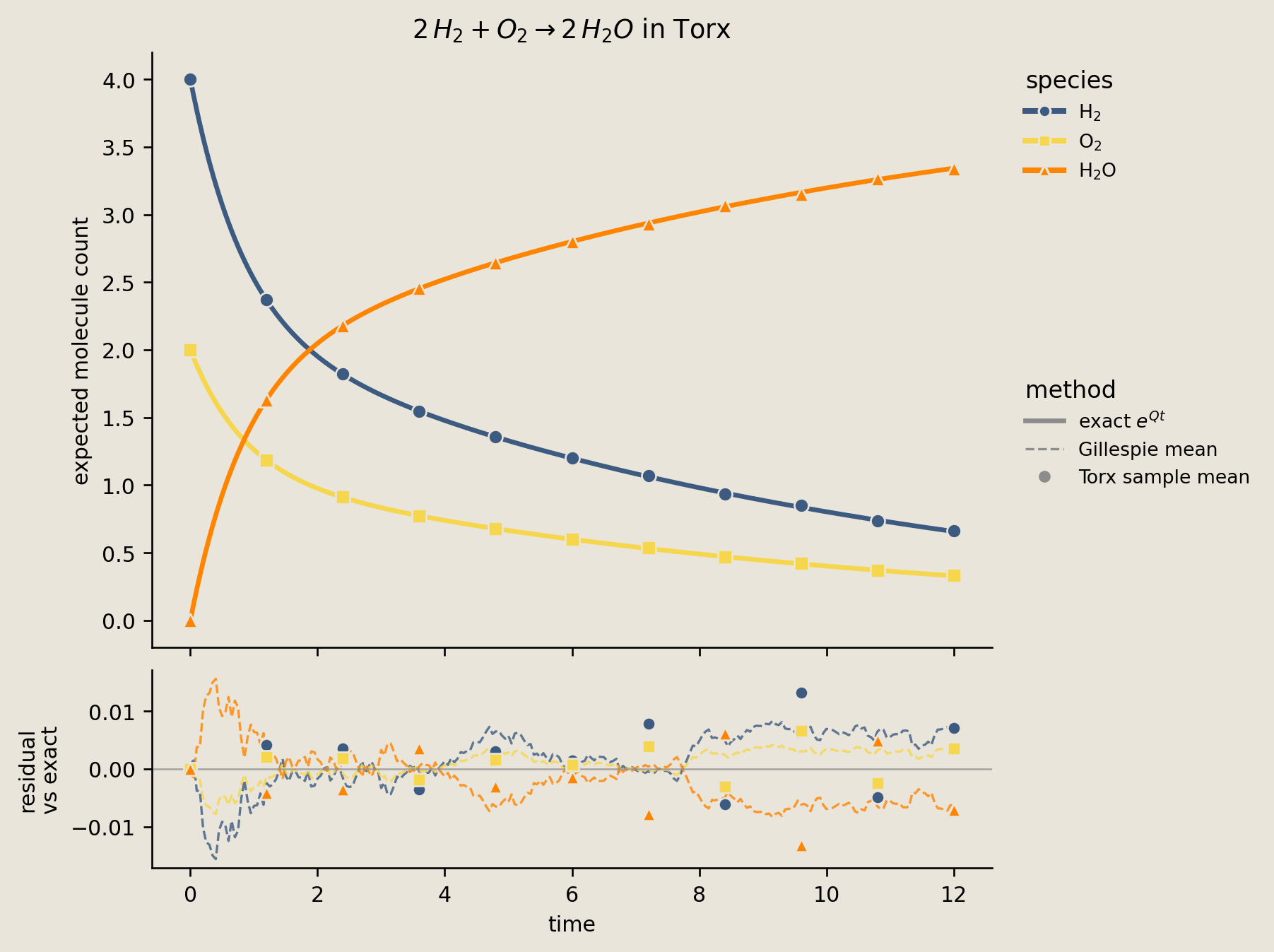
All three count trajectories sit on top of one another at this scale, so the residual panel is where the differences become legible. There the dashed Gillespie means fluctuate around the exact solution because they carry sampling error only, while the shaped Torx markers carry both sampling error and split-step error at each snapshot. The chemistry is visible in the upper panel: $\mathrm{H_2}$ and $\mathrm{O_2}$ are consumed as $\mathrm{H_2O}$ builds up, and the falling propensity slows the reaction as it approaches absorption.
Verification
A faithful configuration-graph encoding must preserve the reaction's chemistry, and all three methods must describe the same chain. We check these requirements separately:
- Stoichiometry. We recompute the H and O atom totals at both endpoints of every reaction edge and require equality. This makes an enumeration error fail directly rather than appear as a small numerical drift.
- Torx against exact. At each snapshot time, we compare the Torx counts with the exact matrix exponential and require the largest absolute deviation to remain below $0.05$. This bound contains the combined split-step and sampling error.
- Gillespie against exact. We apply the same $0.05$ bound to the Gillespie means. Agreement confirms that the raw-count simulation and the configuration-graph solution represent the same reaction.
atoms = {"H": np.array([2, 0, 2]), "O": np.array([0, 2, 1])}
for i, j, _ in config_edges:
    for w in atoms.values():
        assert w @ np.array(configs[i]) == w @ np.array(configs[j])

torx_vs_exact = float(np.max(np.abs(torx_counts - ref_counts[snapshot_reps])))
gil_vs_exact = float(np.max(np.abs(gillespie_counts[snapshot_reps] - ref_counts[snapshot_reps])))
assert torx_vs_exact < 0.05 and gil_vs_exact < 0.05
print(f"atom conservation (H, O)       : OK")
print(f"max |Torx - exact|             : {torx_vs_exact:.4f}  (< 0.05)")
print(f"max |Gillespie - exact|        : {gil_vs_exact:.4f}  (< 0.05)")
print("all checks passed")
atom conservation (H, O)       : OK
max |Torx - exact|             : 0.0132  (< 0.05)
max |Gillespie - exact|        : 0.0065  (< 0.05)
all checks passed
A reversible reaction: binding equilibrium
The water reaction fires in one direction until a reactant is exhausted, so its counts run to completion. We now apply the same encoding to reversible binding, $\mathrm{A} + \mathrm{B} \rightleftharpoons \mathrm{C}$, whose dynamics do not absorb.
The forward reaction $\mathrm{A} + \mathrm{B} \to \mathrm{C}$ has propensity $k_f\,n_{\mathrm{A}}\,n_{\mathrm{B}}$, while the reverse reaction $\mathrm{C} \to \mathrm{A} + \mathrm{B}$ has propensity $k_r\,n_{\mathrm{C}}$. Because both directions remain active, the network relaxes to a stochastic mass-action equilibrium: a steady distribution in which the ensemble forward and reverse fluxes balance. The split-step construction is unchanged, except that the configuration graph now contains edges in both directions.
We define two reactions now, forward and reverse, each with its own rate constant, so the propensity and update helpers take the reaction as an argument instead of reading a single global one. That generalizes the single-reaction versions from the water network without changing what they compute.
A, B, C = 0, 1, 2
species = ["A", "B", "C"]
# two reactions: forward binding A + B -> C (kf), reverse C -> A + B (kr)
kf, kr = 0.18, 0.55
reactions = [
    ({A: 1, B: 1}, {C: 1}, kf),   # forward:  a = kf * nA * nB
    ({C: 1}, {A: 1, B: 1}, kr),   # reverse:  a = kr * nC
]
initial = (4, 4, 0)
def propensity(state, reac, rate):
    """Mass-action propensity of reaction `reac` at `state`."""
    a = rate
    for s, nu in reac.items():
        a *= comb(int(state[s]), nu)
    return a
def apply_reaction(state, reac, prod):
    """Return the configuration after one firing of the (`reac`, `prod`) reaction."""
    out = list(state)
    for s, nu in reac.items():
        out[s] -= nu
    for s, nu in prod.items():
        out[s] += nu
    return tuple(out)
def reachable(initial):
    """Enumerate every configuration reachable from `initial` under all reactions."""
    seen, frontier = {initial}, [initial]
    while frontier:
        s = frontier.pop()
        for reac, prod, rate in reactions:
            if all(s[k] >= nu for k, nu in reac.items()):
                nxt = apply_reaction(s, reac, prod)
                if nxt not in seen:
                    seen.add(nxt); frontier.append(nxt)
    return sorted(seen)
Enumeration follows both directions from here, which means the search reaches each configuration from either side and the configuration graph ends up carrying a forward and a reverse edge between every adjacent pair.
configs_b = reachable(initial)
index_b = {c2: i for i, c2 in enumerate(configs_b)}
edges_b = [
    (index_b[s], index_b[apply_reaction(s, reac, prod)], propensity(s, reac, rate))
    for s in configs_b for reac, prod, rate in reactions
    if all(s[k] >= nu for k, nu in reac.items())
]
print("reachable configurations:", configs_b)
for i, j, rate in edges_b:
    print(f"  {configs_b[i]} -> {configs_b[j]}   propensity = {rate:.3f}")
reachable configurations: [(0, 0, 4), (1, 1, 3), (2, 2, 2), (3, 3, 1), (4, 4, 0)]
  (0, 0, 4) -> (1, 1, 3)   propensity = 2.200
  (1, 1, 3) -> (0, 0, 4)   propensity = 0.180
  (1, 1, 3) -> (2, 2, 2)   propensity = 1.650
  (2, 2, 2) -> (1, 1, 3)   propensity = 0.720
  (2, 2, 2) -> (3, 3, 1)   propensity = 1.100
  (3, 3, 1) -> (2, 2, 2)   propensity = 1.620
  (3, 3, 1) -> (4, 4, 0)   propensity = 0.550
  (4, 4, 0) -> (3, 3, 1)   propensity = 2.880
Because two reactions now compete for the next event, the Gillespie step has to choose which one fires, and it does so with probability proportional to each reaction's propensity.
def gillespie_b(times, n_traj, rng):
    acc = np.zeros((len(times), len(species)))
    for _ in range(n_traj):
        state = np.array(initial); t = 0.0; idx = 0; rec = np.zeros((len(times), len(species)))
        while idx < len(times):
            props = np.array([propensity(state, reac, rate) if all(state[k] >= nu for k, nu in reac.items()) else 0.0
                              for reac, prod, rate in reactions])
            a0 = props.sum()
            if a0 <= 0:
                while idx < len(times): rec[idx] = state; idx += 1
                break
            tau = rng.exponential(1.0 / a0)
            while idx < len(times) and times[idx] < t + tau: rec[idx] = state; idx += 1
            reac, prod, rate = reactions[rng.choice(len(reactions), p=props / a0)]
            state = np.array(apply_reaction(tuple(state), reac, prod)); t += tau
        acc += rec
    return acc / n_traj
We run the exact CTMC and the Gillespie average for the binding network on its own longer time grid, reusing ctmc_reference unchanged so that only the network and the horizon differ.
T_b, N_b = 16.0, 640
dt_b = T_b / N_b
times_b = np.linspace(0.0, T_b, N_b + 1)
p0_b = np.zeros(len(configs_b)); p0_b[index_b[initial]] = 1.0

ref_dist_b, Q_b = ctmc_reference(len(configs_b), edges_b, p0_b, times_b)
ref_counts_b = to_counts(ref_dist_b, configs_b)
gil_counts_b = gillespie_b(times_b, 20_000, np.random.default_rng(SEED))
We build the same sequential split-step circuit for the binding graph, now including the reverse edges, so each slice applies one PJUMP per directed edge and the token can hop either way.
gates_b = [PJUMP([i, j]) for i, j, r in edges_b]
thetas_b = [jnp.array([logit(pjump_prob(r, dt_b))]) for i, j, r in edges_b]
init_bits_b = jnp.zeros(len(configs_b), dtype=jnp.int32).at[index_b[initial]].set(1)
snapshot_reps_b = np.arange(0, N_b + 1, 64, dtype=int)
snapshot_times_b = snapshot_reps_b * dt_b
sim_b = BranchingSimulator(num_samples=30_000)
keys_b = jax.random.split(jax.random.key(SEED), len(snapshot_reps_b))

torx_dist_b = []
for reps, key in zip(snapshot_reps_b, keys_b):
    if reps == 0:
        torx_dist_b.append(np.asarray(init_bits_b, dtype=float))
        continue
    compiled = sim_b.build_circuit(DiscretePCircuit(gates_b, reps=int(reps)), thetas_b)
    torx_dist_b.append(np.asarray(sim_b.sample(compiled, init_bits_b, key)).mean(axis=0))
torx_counts_b = to_counts(np.stack(torx_dist_b), configs_b)
print("evaluated", len(snapshot_reps_b), "snapshots")
evaluated 11 snapshots
As before, the upper panel compares the three count trajectories and the lower panel shows their residuals from the exact solution. Here the long-run comparison is different: equilibrium appears as counts that level off rather than run to completion.
series_b = [
    (r"$\mathrm{A},\ \mathrm{B}$", A, EXACT_COLOR, "o"),
    (r"$\mathrm{C}$", C, TORX_COLOR, "^"),
]
fig = plot_species_dynamics(
    r"$A + B \rightleftharpoons C$ in Torx",
    times_b, ref_counts_b, gil_counts_b, snapshot_times_b, torx_counts_b, series_b,
)
savefig(fig, "05_binding_equilibrium")
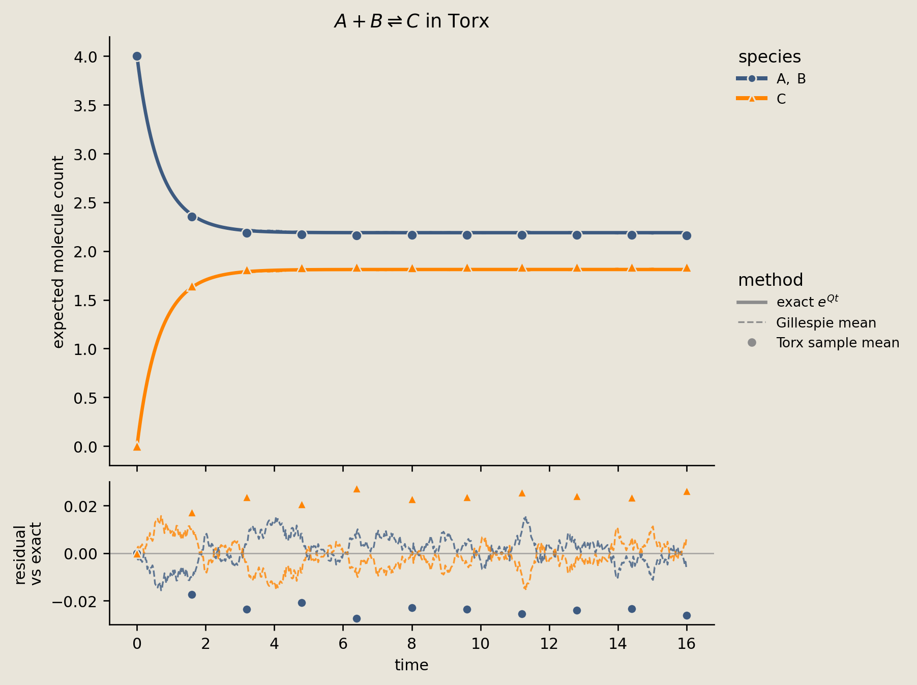
The counts level off well before completion, distinguishing this equilibrium from the absorbing endpoint of the water reaction. $\mathrm{A}$ and $\mathrm{B}$ begin equal and remain equal because $n_{\mathrm{A}} - n_{\mathrm{B}} = 0$ in every reachable configuration, so they follow the same curve. Their means settle near $2.19$, while the mean of $\mathrm{C}$ settles near $1.81$. The residual panel again reveals the small Torx and Gillespie deviations from the exact curves.
The plateaus alone do not specify the equilibrium relation. At stochastic equilibrium, the ensemble fluxes satisfy $k_f\,\mathbb{E}[n_{\mathrm{A}}n_{\mathrm{B}}] = k_r\,\mathbb{E}[n_{\mathrm{C}}]$. This is not equivalent to substituting the mean counts into the rate law.
The same faithfulness question applies to the binding network, with one addition, because a reversible network has something to conserve and something to balance. Binding leaves $n_{\mathrm{A}} + n_{\mathrm{C}}$ and $n_{\mathrm{B}} + n_{\mathrm{C}}$ unchanged, so we recompute both totals at the endpoints of every edge and require them to match, which is the analogue of the atom balance from the water network.
We then repeat the two method comparisons, requiring the largest deviation of the Torx snapshot counts and of the Gillespie means from the exact matrix exponential to stay below $0.05$ at the sampled times.
Finally we test equilibrium directly, evaluating $k_f\,\mathbb{E}[n_{\mathrm{A}}n_{\mathrm{B}}]$ and $k_r\,\mathbb{E}[n_{\mathrm{C}}]$ under the exact distribution at the final time and requiring their difference to fall below $10^{-6}$, so that a pass confirms the plateau in the plot is a genuine flux balance rather than a slow transient.
cons = {"A+C": np.array([1, 0, 1]), "B+C": np.array([0, 1, 1])}
for i, j, _ in edges_b:
    for w in cons.values():
        assert w @ np.array(configs_b[i]) == w @ np.array(configs_b[j])

torx_vs_exact_b = float(np.max(np.abs(torx_counts_b - ref_counts_b[snapshot_reps_b])))
gil_vs_exact_b = float(np.max(np.abs(gil_counts_b[snapshot_reps_b] - ref_counts_b[snapshot_reps_b])))
config_array_b = np.asarray(configs_b)
forward_flux_b = float(kf * np.sum(ref_dist_b[-1] * config_array_b[:, A] * config_array_b[:, B]))
reverse_flux_b = float(kr * np.sum(ref_dist_b[-1] * config_array_b[:, C]))
flux_residual_b = abs(forward_flux_b - reverse_flux_b)

assert torx_vs_exact_b < 0.05 and gil_vs_exact_b < 0.05
assert flux_residual_b < 1e-6
print("conservation (A+C, B+C)        : OK")
print(f"max |Torx - exact|             : {torx_vs_exact_b:.4f}  (< 0.05)")
print(f"max |Gillespie - exact|        : {gil_vs_exact_b:.4f}  (< 0.05)")
print(f"|kf E[n_A n_B] - kr E[n_C]|   : {flux_residual_b:.2e}  (< 1e-6)")
print("all checks passed")
conservation (A+C, B+C)        : OK
max |Torx - exact|             : 0.0274  (< 0.05)
max |Gillespie - exact|        : 0.0105  (< 0.05)
|kf E[n_A n_B] - kr E[n_C]|   : 1.64e-09  (< 1e-6)
all checks passed
The cost: configuration count
The two examples above have small reachable sets, but the encoding width is determined by the number of configurations rather than the number of species. Torx uses one pbit for each reachable configuration, so growth in that count directly increases the circuit width.
For the one-way water family below, only one reaction extent varies and the configuration count grows linearly. The particular water-plus-ammonia family has two independently variable extents, producing quadratic growth. This behavior is not universal: in other networks, conservation laws and feasibility constraints determine which part of the count lattice is reachable.
We count the reachable configurations as the molecule budget grows, first for the single water reaction and then for two reactions that share a species, which is the comparison that separates one free extent from two.
def n_reachable(initial, reaction_list):
    rs = [({a: b for a, b in r[0]}, {a: b for a, b in r[1]}) for r in reaction_list]
    seen, frontier = {initial}, [initial]
    while frontier:
        s = frontier.pop()
        for reac, prod in rs:
            if all(s[k] >= nu for k, nu in reac.items()):
                nxt = list(s)
                for k, nu in reac.items(): nxt[k] -= nu
                for k, nu in prod.items(): nxt[k] += nu
                nxt = tuple(nxt)
                if nxt not in seen: seen.add(nxt); frontier.append(nxt)
    return len(seen)
water = ((( 0, 2), (1, 1)), ((2, 2),))                 # 2 H2 + O2 -> 2 H2O
ammonia = ((( 0, 3), (3, 1)), ((4, 2),))               # N2 + 3 H2 -> 2 NH3
print("one reaction (water), scaling up:")
for k in (2, 4, 8, 16, 32):
    print(f"  H2={2*k:>3}, O2={k:>2}  ->  {n_reachable((2*k, k, 0), [water]):>4} configs")
print("two coupled reactions (water + ammonia, shared H2):")
for k in (2, 4, 8, 16, 32):
    print(f"  H2={6*k:>3}, O2={k:>2}, N2={k:>2}  ->  {n_reachable((6*k, k, 0, k, 0), [water, ammonia]):>4} configs")
one reaction (water), scaling up:
  H2=  4, O2= 2  ->     3 configs
  H2=  8, O2= 4  ->     5 configs
  H2= 16, O2= 8  ->     9 configs
  H2= 32, O2=16  ->    17 configs
  H2= 64, O2=32  ->    33 configs
two coupled reactions (water + ammonia, shared H2):
  H2= 12, O2= 2, N2= 2  ->     9 configs
  H2= 24, O2= 4, N2= 4  ->    25 configs
  H2= 48, O2= 8, N2= 8  ->    81 configs
  H2= 96, O2=16, N2=16  ->   289 configs
  H2=192, O2=32, N2=32  ->  1089 configs
Coupling the second reaction through shared $\mathrm{H_2}$ in this constructed family produces a square grid of reaction extents, which is why the two columns differ by a power rather than by a factor. At the largest budget the water reaction reaches 33 configurations, while this joint network reaches $33^2 = 1089$.
Conclusion
We turned two nonlinear mass-action networks into single-token graph walks by enumerating their reachable configurations, which moves the nonlinearity out of the dynamics and into the edge rates. Torx then applies the per-edge PJUMP kernels as an operator-splitting approximation, while $e^{Qt}$ on the same generator supplies the exact global CTMC reference, so the residual panels separate two distinct disagreements: the combined split-step and sampling error carried by the Torx markers, and the sampling error carried by the Gillespie means.
The price of the one-hot encoding is the reachable configuration count, which grew linearly for the one-reaction family and quadratically for the two-reaction family measured above. Richer encodings become preferable once a network's reachable set grows large. In the linear, single-token corner of this construction the circuit is a directed graph random walk with one walker.
See also:
02_random_walks_on_graphs.ipynb, the single-token graph-transport corner of this construction.04_execution_interface_readouts.ipynb, howBranchingestimates expectations from bitstrings.Simulator
References
- Gillespie, D.T. 1977. Exact stochastic simulation of coupled chemical reactions. J. Phys. Chem. 81(25), 2340-2361. The stochastic simulation algorithm used as a sampling reference above.