
Building a Gaussian hierarchical state-space model
A hidden 3-dimensional drive is visible only through six noisy channels, so we unroll a linear-Gaussian state-space model into affine gates with time-homogeneous parameters, condition on all observations, and read an offline event score that says, at each time step, whether the drive was active. Because that score is allowed to use the whole trial, it comes from the exact smoothed posterior rather than from a running estimate. A dense NumPy recursion plus a Schur complement independently verify the prior propagation and conditioning algebra.
Many systems contain a quantity that matters but cannot be measured directly. Here that quantity is a hidden drive: it rises while an event of interest is under way and falls when the event is absent. We observe only six noisy sensors, each responding to the drive in a different way. Can we use those observations to reconstruct, after the trial is over, the time steps during which the drive was active?
We answer this question with a linear-Gaussian state-space model built in Torx. We begin with the generative model: a 3-dimensional latent state produces six synthetic Gaussian observation channels. We then translate that model into a time-homogeneous circuit, condition on the complete observation sequence, and reduce the inferred state to an event score. This gives one number per time step, near 1 where the model believes the drive was active and near 0 where it believes it was not. Because the data are synthetic, we retain the true latent trajectory and can compare it with the recovered drive at the end.
Each latent state and observation is a pmode, a continuous Torx site valued in $\mathbb{R}^N$ and tracked by its mean and covariance.
The example is time-homogeneous: the same dynamics and emission parameters apply at every time step. Torx represents this assumption by explicitly unrolling the sequence into per-step gates while reusing the same transition and emission theta values.
The resulting program consists of an initial gate, shared-parameter transition gates, and per-step emission gates, all of them Affine instances.
Term: smoothing
Smoothing estimates each latent state from the complete observation sequence, including observations at later time steps. It is therefore an offline, acausal calculation. Filtering is the online counterpart: it estimates the state at each step using only that step's observation and earlier observations, so it can run as data arrives. We use smoothing because the trial is complete and we want the best estimate at every step rather than a causal estimate.
By the end, you'll be able to:
- build one initial gate, one gate per transition, and one per emission,
- condition on all observations to get the exact smoothed posterior, equivalent to Kalman filtering (1960) followed by Rauch-Tung-Striebel smoothing (1965), and
- run a one-seed sanity check that the smoother recovered the hidden drive, using a dense NumPy prior recursion and conditioning formula as the reference.
Setup
We import the dependencies and define one small helper, _det_log_var, which returns the log-variance of a noise-free affine channel so that deterministic passthrough coordinates get exact zero variance instead of a small positive one.
What runs where?
- Torx gates build the joint Gaussian and compute the exact smoothed posterior.
- Notebook code generates the Gaussian observations, implements the dense reference, and computes the uncalibrated score.
examples/helpers/_plots_fields.pyandexamples/helpers/_plots_schematics.pyrender the supplied arrays and circuit semantics.examples/helpers/_notebook_paths.pyandexamples/helpers/_notebook_style.pymanage offline figure paths and style.
from pathlib import Path
import sys

import jax.numpy as jnp
import numpy as np
ROOT = Path.cwd()
if not (ROOT / "helpers").exists() and (ROOT.parent / "helpers").exists():
    ROOT = ROOT.parent
HELPER_DIR = ROOT / "helpers"
sys.path.insert(0, str(HELPER_DIR))
from _notebook_paths import figure_dir
from _notebook_style import apply_notebook_style, make_savefig
import _plots_fields as P_fld
import _plots_schematics as P_sch
from torx.psc import AffineGaussianGate, HybridPCircuit
apply_notebook_style()
FIGURE_DIR = figure_dir(ROOT)
SEED = 23
rng = np.random.default_rng(SEED)


savefig = make_savefig(FIGURE_DIR)
def _det_log_var(dim):
    """Log-variance of a noise-free (deterministic) affine channel."""
    return jnp.full((dim,), -jnp.inf)
The model
Before we build anything we need to state exactly what generates the data, because every gate in the next section is a direct translation of one line of the equations below.
A 3-dimensional latent state (latent_dim = 3) carries the hidden drive, and the six synthetic Gaussian observation channels (num_channels = 6) that we actually get to see are generated directly by the observation equation below.
The model is linear-Gaussian:
$$ z_0 \sim \mathcal{N}(m_0,\,P_0),\qquad z_t = \underbrace{A\,z_{t-1}}_{\vphantom{\big|}\text{drift}} + \underbrace{\varepsilon_t}_{\vphantom{\big|}\text{process noise}}, $$ $$ x_t = C\,z_t + \eta_t. $$
The initial state draws from the prior $\mathcal{N}(m_0,P_0)$, the process noise is $\varepsilon_t \sim \mathcal{N}(0,Q)$, the measurement noise is $\eta_t \sim \mathcal{N}(0,R)$, and $C$ is the observation map.
Nothing on either right-hand side depends on $t$, so a single set of parameters describes the whole sequence. The transition sub-product makes that reuse explicit by using the same transition parameters at every adjacent pair:
$$ G_{\mathrm{trans}}(\theta)=\underbrace{\prod_{t=1}^{T-1}}_{\vphantom{\big|}\text{$T-1$ transitions}} \underbrace{K_\theta^{(t-1,\,t)}}_{\vphantom{\big|}\text{same theta reused}} . $$
Each factor $K_\theta^{(t-1,\,t)}$ is the transition kernel from latent site $t-1$ to latent site $t$, and every transition gate reuses the same fixed theta values while the built circuit stays explicitly unrolled into one gate per transition and one gate per emission.
The initial gate carries the prior $\mathcal{N}(m_0,P_0)$, and the emission gates carry the observation map $C$ and the measurement noise $R$. One length-$T$ sequence is therefore one initial gate, $T-1$ transition gates that reuse the same transition theta, and $T$ emission gates that reuse the same emission theta.
First we fix the size of the problem: how many time steps there are, how wide the latent state is, and how many channels observe it. The same cell fixes intent_axis, the direction in latent space along which we read the drive as a single number, because both the hidden labels and the score later project onto it.
T = 32
latent_dim = 3
num_channels = 6

latent_sites = list(range(T))
obs_sites = list(range(T, 2 * T))
intent_axis = np.array([1.0, 0.35, -0.25])
The transition matrix A specifies the latent dynamics from one time step to the next, which makes it the only part of the model that carries information forward in time.
A = np.array(
    [
        [0.92, 0.08, 0.00],
        [-0.04, 0.88, 0.06],
        [0.02, -0.08, 0.90],
    ]
)
The observation matrix C maps the latent state into six continuous channels, one row per channel. Every row mixes all three latent coordinates, so no single channel is a clean view of the drive.
C = np.array(
    [
        [1.15, 0.10, -0.15],
        [0.85, -0.25, 0.05],
        [-0.35, 0.95, 0.20],
        [0.20, 0.45, 0.85],
        [-0.10, -0.55, 1.05],
        [0.55, 0.15, -0.65],
    ]
)
What remains are the scales that decide how hard the recovery problem is. The prior mean m0 and the diagonal covariance parameters set the initial uncertainty (P0_diag), the process noise that perturbs the latent state at every step (Q_diag), and the measurement noise added to each channel (R_diag).
m0 = np.array([-0.45, 0.15, 0.10])
P0_diag = np.array([0.35, 0.25, 0.20])
Q_diag = np.array([0.055, 0.045, 0.040])
R_diag = np.array([0.16, 0.18, 0.20, 0.17, 0.19, 0.16])
With every parameter fixed we can generate a trial. simulate_lgssm draws one latent trajectory and six Gaussian observation channels with plain NumPy, following the two model equations line for line.
def simulate_lgssm():
    z = np.zeros((T, latent_dim))
    x = np.zeros((T, num_channels))
    # Draw the prior state and its first noisy observation.
    z[0] = rng.multivariate_normal(m0, np.diag(P0_diag))
    x[0] = C @ z[0] + rng.normal(scale=np.sqrt(R_diag))
    for t in range(1, T):
        # Reuse the same dynamics and noise scale at each later step.
        z[t] = A @ z[t - 1] + rng.normal(scale=np.sqrt(Q_diag))
        x[t] = C @ z[t] + rng.normal(scale=np.sqrt(R_diag))
    return z, x
Running it once gives us both halves of the experiment: a synthetic Gaussian trial whose observations we condition on, and the hidden true_event labels that we set aside for the one-seed sanity check at the end.
true_latent, observations = simulate_lgssm()
true_drive = true_latent @ intent_axis

true_event_threshold = 0.0
true_event = true_drive > true_event_threshold
true_event_rate = float(true_event.mean())
majority_baseline_acc = max(true_event_rate, 1.0 - true_event_rate)

print(f"T={T}, latent_dim={latent_dim}, num_channels={num_channels}")
print(f"true events active: {true_event.sum()} / {T}  (rate = {true_event_rate:.1%})")
print(f"majority-class baseline accuracy: {majority_baseline_acc:.1%}")
T=32, latent_dim=3, num_channels=6
true events active: 12 / 32  (rate = 37.5%)
majority-class baseline accuracy: 62.5%
A shape check catches simulation mistakes here, while the arrays are still readable, instead of later as a dimension error inside the circuit.
np.testing.assert_equal(true_latent.shape, (T, latent_dim))
np.testing.assert_equal(observations.shape, (T, num_channels))
The printed true_event_rate also fixes majority_baseline_acc, the accuracy you would reach by always guessing the more common class. That's the bar the score has to clear in the detector comparison later, since beating it is the minimum evidence that the posterior carries real information about the drive.
Building the circuit
Now we turn those equations into gates. Each time index has one latent pmode and one observation pmode, and every gate writes one new site while copying the site it read.
The transition gates implement the kernel $K_\theta^{(t-1,\,t)}$ above, and the initial and emission gates carry the prior and the observation model:
- Initial gate ($t=0$): encodes the prior $z_0 \sim \mathcal{N}(m_0, P_0)$ as a single-site
Affine.Gaussian Gate - Transition gate ($t=1\ldots T-1$): uses a block matrix that copies $z_{t-1}$ and writes $z_t = A z_{t-1}$, with process noise $Q$ on the new site.
- Emission gate ($t=0\ldots T-1$): uses a block matrix that copies $z_t$ and writes $x_t = C z_t$, with measurement noise $R$ on the observation site.
Passthrough coordinates take log_var = -inf via the visible _det_log_var helper above, which is what makes them exact deterministic copies. The block structure carries the model, and the gate list repeats it across time by aliasing the same fixed theta.
Both gate types work the same way, so we build their matrices together. The matrices transition_matrix and emission_matrix make the deterministic passthrough coordinates explicit, which is what lets a single affine gate both copy a site and write the next one beside it.
# First block copies z_{t-1}; second block writes the next latent state.
transition_matrix = np.block(
    [
        [np.eye(latent_dim), np.zeros((latent_dim, latent_dim))],
        [A, np.zeros((latent_dim, latent_dim))],
    ]
)

# First block keeps z_t; second block writes the predicted observation.
emission_matrix = np.block(
    [
        [np.eye(latent_dim), np.zeros((latent_dim, num_channels))],
        [C, np.zeros((num_channels, num_channels))],
    ]
)
The first gate has nothing to read from, so initial_gate simply writes the Gaussian prior onto the first latent site.
initial_gate = AffineGaussianGate(
    sites=[latent_sites[0]],
    dims=(latent_dim,),
)
initial_theta = {
    "A": jnp.zeros((latent_dim, latent_dim)),
    "b": jnp.asarray(m0),
    "log_var": jnp.log(jnp.asarray(P0_diag)),
}
Next come the transitions. The transition gates in transition_gates unroll adjacent time steps, and each one aliases the same transition parameter dictionary rather than owning a copy of it.
That sharing is inference-time reuse of the same fixed theta values, not trainable parameter tying, and no compact scan primitive is involved. Under a normal JAX optimizer the repeated gates would receive separate gradients, so training would require an explicit gate-to-theta reduction. The passthrough coordinates are the second obstacle: log_var = -inf is exact for conditioning but not differentiable through those coordinates, so clamp it to a large finite-negative value before training with gradients.
transition_gates = [
    AffineGaussianGate(
        sites=[latent_sites[t - 1], latent_sites[t]],
        dims=(latent_dim, latent_dim),
    )
    for t in range(1, T)
]
transition_theta = {
    "A": jnp.asarray(transition_matrix),
    "b": jnp.zeros(2 * latent_dim),
    "log_var": jnp.concatenate(
        [
            _det_log_var(latent_dim),
            jnp.log(jnp.asarray(Q_diag)),
        ]
    ),
}
transition_thetas = [transition_theta for _ in range(1, T)]
Emissions follow the same pattern in the other direction, so the emission gates in emission_gates attach one observed pmode to each latent time step.
emission_gates = [
    AffineGaussianGate(
        sites=[latent_sites[t], obs_sites[t]],
        dims=(latent_dim, num_channels),
    )
    for t in range(T)
]
emission_theta = {
    "A": jnp.asarray(emission_matrix),
    "b": jnp.zeros(latent_dim + num_channels),
    "log_var": jnp.concatenate(
        [
            _det_log_var(latent_dim),
            jnp.log(jnp.asarray(R_diag)),
        ]
    ),
}
emission_thetas = [emission_theta for _ in range(T)]
Hybrid combines the gate groups into the full unrolled circuit. The parameters stay outside it, one theta per gate collected in a matching list, which is why thetas has to be exactly as long as circuit.gates.
circuit = HybridPCircuit([initial_gate, *transition_gates, *emission_gates])
# Parameters live outside the circuit, one theta per gate in gate order.
thetas = [initial_theta, *transition_thetas, *emission_thetas]
np.testing.assert_equal(len(thetas), len(circuit.gates))

print(f"{len(circuit.gates)} AffineGaussianGate instances")
print(f"  1 initial + {T - 1} transition + {T} emission = {1 + (T - 1) + T}")
64 AffineGaussianGate instances
  1 initial + 31 transition + 32 emission = 64
A site layout this repetitive is easy to get wrong by one, so a dimension check confirms the latent and observed site layout in circuit before anything reads from it.
np.testing.assert_equal(circuit.continuous_dims, (latent_dim,) * T + (num_channels,) * T)
The printed count confirms that one initial gate, 31 transition gates, and 32 emission gates represent the model.
One time slice contains a transition followed by an emission, and because the other 31 slices repeat it exactly, we draw that slice once as a directed schematic.
fig_c = P_sch.plot_ssm_slice_circuit()
savefig(fig_c, "11_ssm_slice_circuit")
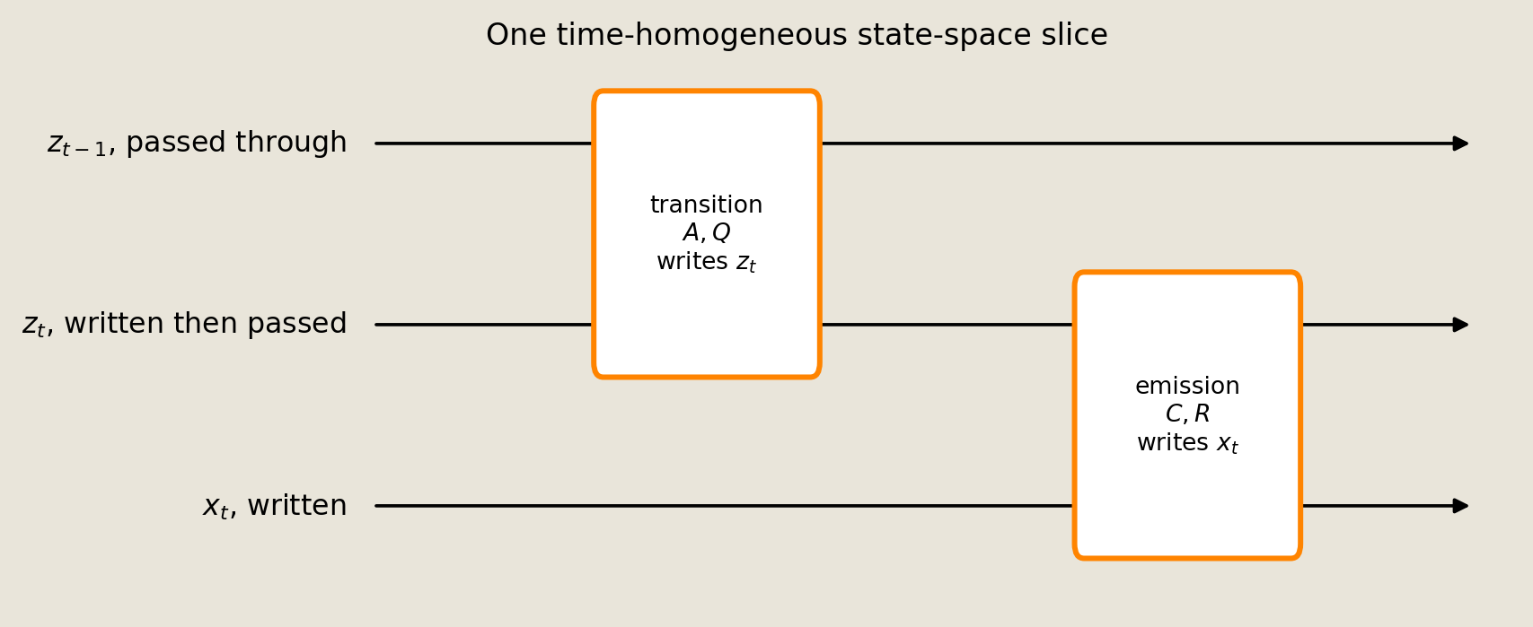
Reading the schematic left to right, the slice writes $z_t$ with the transition parameters $A,Q$, then writes $x_t$ with the emission parameters $C,R$, while the labeled passthrough wires carry the source coordinates through untouched.
Exact posterior
With the joint Gaussian assembled, we can infer the latent drive from the observations. For this linear-Gaussian model, conditioning on the complete observation sequence is exact: it gives the same smoothed posterior as the classical two-pass recursion. Kalman filtering (1960) first moves forward through the data to compute a causal estimate at each step; Rauch, Tung, and Striebel smoothing (1965) then moves backward to revise those estimates using later observations.
AffineGaussianSimulator.condition obtains the same result by conditioning on all 32 observations at once. Because every latent estimate can use later observations, the result is offline and acausal as well as exact for this model.
We therefore compile the circuit for Affine, supply the observed pmodes in observed, and query the latent pmodes in latent_sites.
observed = {site: jnp.asarray(observations[t]) for t, site in enumerate(obs_sites)}
from torx.psc import AffineGaussianSimulator
affine_sim = AffineGaussianSimulator()
compiled = affine_sim.build_circuit(circuit, thetas)

# flat initial continuous state over all latent + observed sites
initial_continuous = jnp.zeros(T * latent_dim + T * num_channels)
# Condition on observed sites, then return moments only for the latent sites.
posterior = affine_sim.condition(
    compiled,
    observations=observed,
    initial_continuous=initial_continuous,
    query_sites=latent_sites,
)
posterior_mean = np.asarray(posterior.mean).reshape(T, latent_dim)
posterior_cov = np.asarray(posterior.covariance)
The exactness claim needs a reference that does not reuse the gate construction. A dense NumPy baseline independently propagates the LGSSM moments from (A, C, Q, R, m0, P0) and applies the Schur-complement conditioning formula. This separates two checks: Torx must reproduce both the dense prior propagation and the dense posterior, within the relative and absolute tolerances asserted below.
def dense_lgssm_joint_moments(A, C, m0, P0_diag, Q_diag, R_diag, T):
    A = np.asarray(A, dtype=float)
    C = np.asarray(C, dtype=float)
    m0 = np.asarray(m0, dtype=float)
    Q = np.diag(np.asarray(Q_diag, dtype=float))
    R = np.diag(np.asarray(R_diag, dtype=float))
    latent_dim = A.shape[0]
    num_channels = C.shape[0]

    z_mean = np.zeros((T, latent_dim))
    z_cov = np.zeros((T, T, latent_dim, latent_dim))
    z_mean[0] = m0
    z_cov[0, 0] = np.diag(np.asarray(P0_diag, dtype=float))
    for t in range(1, T):
        z_mean[t] = A @ z_mean[t - 1]
        for s in range(t):
            cov_ts = A @ z_cov[t - 1, s]
            z_cov[t, s] = cov_ts
            z_cov[s, t] = cov_ts.T
        z_cov[t, t] = A @ z_cov[t - 1, t - 1] @ A.T + Q

    total_dim = T * latent_dim + T * num_channels
    mean = np.zeros(total_dim)
    cov = np.zeros((total_dim, total_dim))
    obs_mean = z_mean @ C.T
    mean[: T * latent_dim] = z_mean.reshape(-1)
    mean[T * latent_dim :] = obs_mean.reshape(-1)

    def z_slice(t):
        return slice(t * latent_dim, (t + 1) * latent_dim)

    def x_slice(t):
        start = T * latent_dim + t * num_channels
        return slice(start, start + num_channels)

    for t in range(T):
        for s in range(T):
            cov_zz = z_cov[t, s]
            cov[z_slice(t), z_slice(s)] = cov_zz
            cov[z_slice(t), x_slice(s)] = cov_zz @ C.T
            cov[x_slice(t), z_slice(s)] = C @ cov_zz
            cov_xx = C @ cov_zz @ C.T
            if t == s:
                cov_xx = cov_xx + R
            cov[x_slice(t), x_slice(s)] = cov_xx
    return mean, cov
First, propagate the Torx prior through every site and check it against the dense joint moments. Testing the prior on its own isolates the propagation algebra, so a failure here can't be blamed on the conditioning step.
prior = affine_sim.propagate(compiled, initial_continuous)
dense_prior_mean, dense_prior_cov = dense_lgssm_joint_moments(
    A, C, m0, P0_diag, Q_diag, R_diag, T
)
np.testing.assert_equal(prior.sites, tuple(latent_sites + obs_sites))
np.testing.assert_allclose(prior.mean, dense_prior_mean, rtol=1e-5, atol=3e-5)
np.testing.assert_allclose(prior.covariance, dense_prior_cov, rtol=1e-5, atol=3e-5)
Then condition the dense joint on the same observations. The Schur complement gives the reference posterior mean and covariance for the Torx result to match, and the assertion below confirms that it does, to a relative tolerance of 1e-5.
latent_total = T * latent_dim
query_idx = np.arange(latent_total)
obs_idx = np.arange(latent_total, latent_total + T * num_channels)
y = observations.reshape(-1)
# condition returns query_sites in latent_sites order, matching query_idx.
Soo = dense_prior_cov[np.ix_(obs_idx, obs_idx)]
Sqo = dense_prior_cov[np.ix_(query_idx, obs_idx)]
Sqq = dense_prior_cov[np.ix_(query_idx, query_idx)]
dense_mean = dense_prior_mean[query_idx] + Sqo @ np.linalg.solve(
    Soo, y - dense_prior_mean[obs_idx]
)
dense_cov = Sqq - Sqo @ np.linalg.solve(Soo, Sqo.T)
np.testing.assert_allclose(posterior.mean, dense_mean, rtol=1e-5, atol=3e-5)
np.testing.assert_allclose(posterior.covariance, dense_cov, rtol=1e-5, atol=3e-5)
np.testing.assert_equal(posterior_mean.shape, (T, latent_dim))
np.testing.assert_array_less(-1e-6, np.linalg.eigvalsh(posterior_cov))
Exact agreement establishes the posterior values, but the covariance should also reflect the local dynamics. We divide the smoothed covariance into per-timestep blocks and test two expectations: most of the mass should lie on the diagonal, and the nearest-neighbor lag should be the largest off-diagonal term. The printed mean block norms for lags 0 through 4 make that comparison visible.
block_norms = np.array(
    [
        [
            np.linalg.norm(
                posterior_cov[
                    t * latent_dim : (t + 1) * latent_dim,
                    s * latent_dim : (s + 1) * latent_dim,
                ]
            )
            for s in range(T)
        ]
        for t in range(T)
    ]
)
lag_mean_norms = np.array(
    [np.mean([block_norms[t, t + lag] for t in range(T - lag)]) for lag in range(T)]
)
offdiag_lag_means = lag_mean_norms[1:]
np.testing.assert_equal(int(np.argmax(offdiag_lag_means)), 0)
np.testing.assert_array_less(np.mean(lag_mean_norms[4:]), lag_mean_norms[1])
print(f"mean block norms by lag 0..4: {lag_mean_norms[:5].round(4).tolist()}")
mean block norms by lag 0..4: [0.056699998676776886, 0.027799999341368675, 0.014000000432133675, 0.0071000000461936, 0.003700000001117587]
A single number summarizes how well the model explains this trial at all. The next cell computes the model log-evidence from the dense reference: the log-probability of the observed data under the model, with the latent states marginalized away.
# Soo is an SPD observation covariance, so take its log-det from the Cholesky
# factor: the stable SPD path, and it raises LinAlgError if Soo is ever not
# positive definite instead of returning a quietly wrong number.
chol_Soo = np.linalg.cholesky(Soo)
logdet = float(2.0 * np.sum(np.log(np.diag(chol_Soo))))
y_centered = y - dense_prior_mean[obs_idx]
log_evidence = float(
    -0.5
    * (
        len(y) * np.log(2 * np.pi)
        + logdet
        + y_centered @ np.linalg.solve(Soo, y_centered)
    )
)
print("Torx matches the independent dense LGSSM baseline")
print(f"log-evidence: {log_evidence:.3f}")
Torx matches the independent dense LGSSM baseline
log-evidence: -152.580
The printed log_evidence scores this observed trial under the dense reference model. It only means something in comparison, so compare candidate models only on the same observations and with the same likelihood conventions.
Offline event-score sanity check
Agreement with the dense reference establishes the inference algebra. We now ask a different question: did the smoother recover the hidden drive in this trial? We project posterior_mean onto intent_axis, reducing each 3-dimensional smoothed state to the scalar drive of interest. Projecting each per-site covariance marginal along the same direction gives the variance of that scalar, so every estimate has an associated uncertainty.
Two constraints limit the conclusion. First, intent_axis is fixed in advance and also defines the hidden labels, so the score and labels are read along the same direction. Second, the experiment uses a single seed. This is therefore a check that the circuit and conditioning recover a latent signal, not an estimate of detector performance on data for which the scoring direction was unknown.
The binary prediction uses the median of the complete smoothed trajectory as its threshold. Both the threshold and the smoothed posterior use future time bins, so this is a retrospective full-trial analysis rather than an online procedure.
We begin by computing the posterior drive posterior_drive and its standard deviation posterior_drive_std from the smoothed latent moments.
posterior_drive = posterior_mean @ intent_axis
posterior_drive_var = np.array(
    [
        # Project each smoothed covariance onto the same one-dimensional intent axis.
        intent_axis @ np.asarray(posterior.site_moments(s)[1]) @ intent_axis
        for s in latent_sites
    ]
)
posterior_drive_std = np.sqrt(np.maximum(posterior_drive_var, 0.0))
We convert the drive to an uncalibrated display score with a logistic transform centered on the full-trial median. The score preserves the ordering of the drive but is not a probability, and its 0.5 decision boundary is exactly posterior_drive > detection_threshold.
detection_threshold = float(np.median(posterior_drive))
# Center the logistic display score at the median; the decision is the same threshold on posterior_drive.
event_score = 1.0 / (1.0 + np.exp(-3.0 * (posterior_drive - detection_threshold)))
predicted_event = posterior_drive > detection_threshold
For this one seeded check on the oracle axis, we summarize latent-drive recovery with accuracy, AUC (the chance that a randomly chosen active step scores above a randomly chosen inactive one), precision, recall, and confusion counts, all of which describe this one synthetic trial and nothing beyond it.
accuracy = float(np.mean(predicted_event == true_event))

pos = posterior_drive[true_event]
neg = posterior_drive[~true_event]
# AUC and precision/recall are undefined without both classes present.
assert pos.size and neg.size, "metrics require both event and non-event steps"
# tie-aware AUC (Mann-Whitney): ties between a positive and negative get half credit
gt = float((pos[:, None] > neg[None, :]).mean())
eq = float((pos[:, None] == neg[None, :]).mean())
auc = gt + 0.5 * eq
tp = int(np.sum(predicted_event & true_event))
fp = int(np.sum(predicted_event & ~true_event))
fn = int(np.sum(~predicted_event & true_event))
# report undefined metrics as nan rather than masking an empty denominator
precision = tp / (tp + fp) if (tp + fp) else float("nan")
recall = tp / (tp + fn) if (tp + fn) else float("nan")
if accuracy < majority_baseline_acc + 0.05:
    raise AssertionError(
        f"detector accuracy {accuracy:.2%} barely beats majority "
        f"({majority_baseline_acc:.2%}); posterior isn't informative enough."
    )
if auc < 0.80:
    raise AssertionError(f"posterior-drive AUC {auc:.2f} below 0.80")
print(f"full-trial median threshold: {detection_threshold:.4f}")
print(
    f"one-seed oracle-axis accuracy: {accuracy:.1%}  "
    f"(vs majority baseline {majority_baseline_acc:.1%})"
)
print(f"AUC: {auc:.3f}")
print(f"precision: {precision:.2f}   recall: {recall:.2f}")
full-trial median threshold: -0.0654
one-seed oracle-axis accuracy: 81.2%  (vs majority baseline 62.5%)
AUC: 0.921
precision: 0.69   recall: 0.92
confusion counts: TP=11, FP=5, FN=1, TN=15
All of these numbers describe one seeded synthetic trajectory scored along the same oracle axis that defined its labels, so they confirm that the circuit recovers the drive rather than showing what a detector would do in general.
It helps to see what the model has to work with before looking at what it recovered. The first plot shows the six synthetic Gaussian observation channels, with gray bands on time steps where the true drive is positive.
fig = P_fld.plot_observations(observations, true_event)
savefig(fig, "11_ssm_observations")
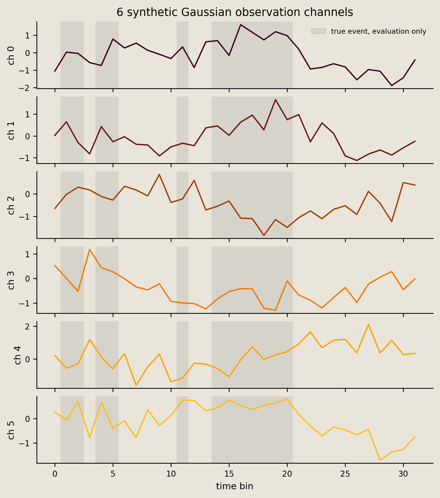
Each trace corresponds to a different row of C, so the drive appears with different signs and amplitudes across the six channels. No channel is a clean view on its own. The gray bands show the active event steps, which are used only for evaluation.
Now we put the recovered drive next to the truth. The next plot compares true_drive with the offline Torx-smoothed posterior_drive, both projected onto intent_axis. It also shows the $\pm 2\sigma$ marginal band and the dashed full-trial median threshold.
The smoother and threshold use the complete 32-step trial.
fig = P_fld.plot_posterior_drive(
    true_drive,
    posterior_drive,
    posterior_drive_std,
    detection_threshold,
)
savefig(fig, "11_ssm_posterior_drive")
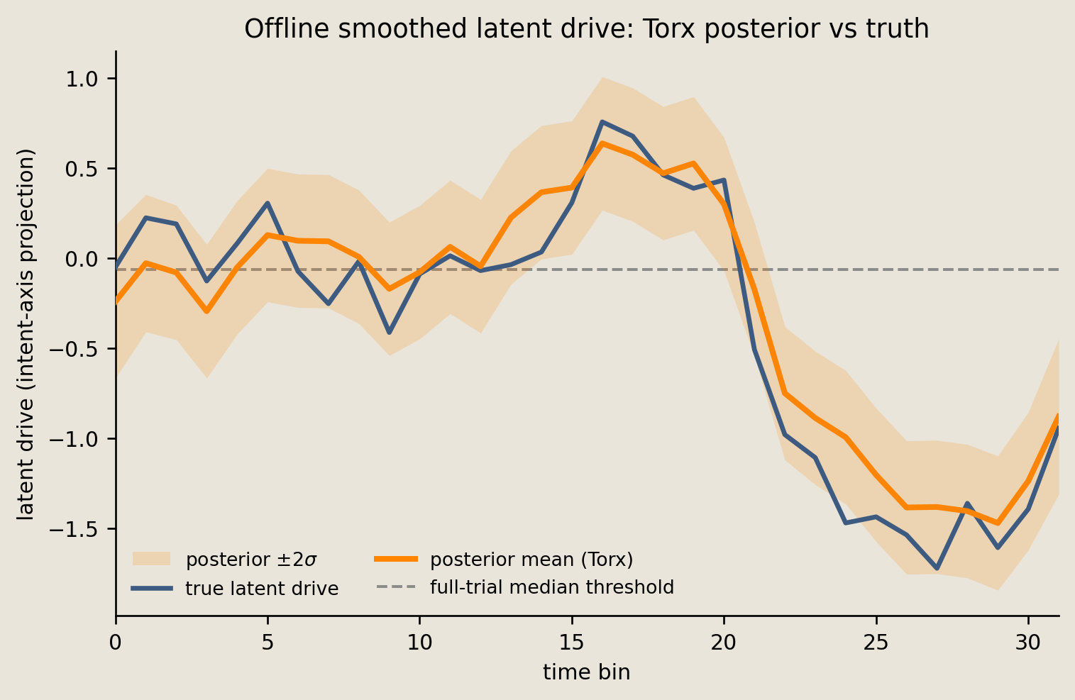
The posterior mean tracks the latent drive in this seeded trial, and the marginal uncertainty widens near the boundaries, where fewer observations surround a latent state.
The last structural question is how far across time the posterior ties states together. The covariance plot shows the Frobenius norm of each $3 \times 3$ timestep block, so diagonal cells describe same-step uncertainty and any bright off-diagonal band means the smoother has linked states that far apart.
fig = P_fld.plot_posterior_covariance(block_norms)
savefig(fig, "11_ssm_covariance")
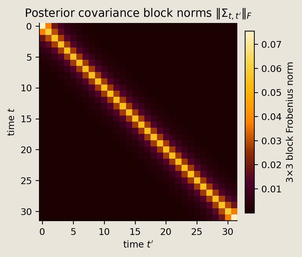
The block-norm covariance remains concentrated near the diagonal, with the nearest-neighbor band the strongest off-diagonal coupling and longer-lag block norms smaller, matching the lag means printed in the check above. That's what local time-homogeneous dynamics should produce.
Finally we look at the score itself. The last plot shows the uncalibrated offline score and the resulting binary event bars for this one-seed oracle-axis sanity check.
time = np.arange(T)
fig = P_fld.plot_detector(time, event_score, true_event, predicted_event, accuracy)
savefig(fig, "11_ssm_detector")
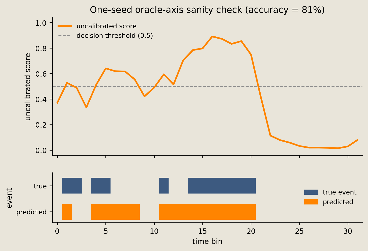
The predicted bars align with most active intervals, at the accuracy printed above for this seeded oracle-axis check.
Conclusion
We began with a hidden drive observed through six noisy channels. A time-homogeneous linear-Gaussian model specified how that drive generated the observations; an explicitly unrolled Torx circuit represented the model; exact conditioning recovered the smoothed latent trajectory; and the final diagnostics compared that trajectory with the known synthetic truth.
- The model is represented as 64
Affineinstances, one initial gate plus one gate per transition and emission.Gaussian Gate - Transition and emission gates alias fixed
thetadictionaries at inference time while the circuit remains explicitly unrolled, which keeps the sharing free to build but explicit to train. AffineGaussianSimulator.conditionreturns the exact offline, acausal smoothed posterior and matches the dense NumPy reference to a relative tolerance of1e-5.- The median-threshold metrics are a one-seed oracle-axis sanity check, because the axis that scores the drive is the axis that defined the labels, and the logistic output is an uncalibrated score.
- Exact
-infpassthrough log-variances are what make the conditioning exact here, but they must be clamped before gradient training.
This tutorial applies the affine-Gaussian density layer of 10_pmode_gaussian_gates.ipynb to a time series. To continue, work through 12_langevin_graph_ising.ipynb.
References
- Kalman, R.E. 1960. A new approach to linear filtering and prediction problems. Trans. ASME J. Basic Eng. 82(1), 35-45.
- Rauch, H.E., Tung, F., Striebel, C.T. 1965. Maximum likelihood estimates of linear dynamic systems. AIAA J. 3(8), 1445-1450.