
Training a stochastic graph network for MaxCut
We train a graph circuit for MaxCut, the problem of splitting a graph's nodes into two groups so that as many edges as possible run between the groups. One sweep applies 12 sequential PISING edge updates, and the circuit repeats that sweep 20 times. Training uses REINFORCE, which raises the probability of the sampled partitions that cut more edges than the batch average, and because the graph has only 8 nodes the exact Torx simulator supplies and differentiates the full probability vector behind every score.
In this tutorial, we ask how an edge-local stochastic circuit can learn a global graph partition. The example is MaxCut: split a graph's nodes into two groups so that as many edges as possible have one endpoint in each group. The number of crossing edges is the cut value we seek to maximize.
We place one probabilistic bit (p-bit), a Bernoulli-valued state, on each graph node. Its value records which of the two groups the node currently belongs to. The circuit then places one edge-local PISING gate on each of the graph's 12 edges. A sweep applies these 12 gates sequentially in fixed edge-list order, and the circuit repeats the sweep 20 times.
The difficulty is that the cut of one sampled partition is a discrete count, not a differentiable function of the couplings. We therefore use the REINFORCE gradient estimator (Williams 1992), which learns from a distribution by sampling from it, scoring each sample, and increasing the probability of samples that score above the batch average. Here, State computes the exact 256-entry probability vector, sampling uses that vector, and JAX differentiates its exact log probabilities.
This tutorial uses Torx, JAX, Optax, and NumPy, with NetworkX behind the graph helper, and assumes basic graph and probability notation.
What runs where?
- Torx:
Statecomputes the full classical probability vector for the 8-node circuit.Vector Simulator - Notebook code: JAX differentiates exact log probabilities in the REINFORCE surrogate, and Optax applies Adam updates.
- Computational helper:
examples/helpers/_nb09_maxcut.pybuilds the circuit, exact diagnostic, graph reference, and result figures. - Plot helper:
examples/helpers/_plots_schematics.pydraws the edge-local circuit primitive.
By the end, you'll be able to:
- build a circuit with 12 sequential
PISINGedge updates per sweep and repeat it for 20 sweeps, - estimate the expected-cut gradient from sampled bitstrings, using the batch's own mean cut as the baseline, and
- train the edge couplings so the circuit puts more probability on high-cut partitions.
A stochastic graph network is an edge-tiled message-passing circuit.
- Each edge carries one learnable coupling $J_{ij}$.
- Each
PISINGkernel is an edge update: a $4\times4$ column-stochastic Markov matrix, meaning each column of probabilities sums to one. It pushes its two endpoints toward agreement when $J>0$ and disagreement when $J<0$. - One sweep applies all 12 edge updates sequentially in fixed order. Repeating sweeps makes the network deeper.
- The readout is the cut value, the number of edges whose endpoints disagree.
- Training raises the expected cut.
The quantity we want to raise is an average over sampled bitstrings, and the cut of any one bitstring is a discrete count, which is the situation REINFORCE was designed for. It scores each sampled bitstring by its cut, subtracts the mean cut of the same batch as a baseline, and uses the difference to weight the gradient of that sample's log probability, so partitions that beat the batch average become more likely and the rest become less likely. Subtracting a baseline that those same samples produced would bias the estimate slightly, so we scale the result by a small correction factor that removes the bias exactly. We write the estimator out in full where the training loop implements it. An optax optimizer then applies the updates.
Setup
The setup cells wire up the helper path and apply the shared figure style. The MaxCut utilities come from examples/helpers/_nb09_maxcut.py.
from pathlib import Path
import sys

import numpy as np
import jax
import jax.numpy as jnp
import optax

from torx.psc import DiscretePCircuit, PISING
ROOT = Path.cwd()
if not (ROOT / "helpers").exists() and (ROOT.parent / "helpers").exists():
    ROOT = ROOT.parent
HELPER_DIR = ROOT / "helpers"
sys.path.insert(0, str(HELPER_DIR))
from _notebook_paths import figure_dir
from _notebook_style import apply_notebook_style, make_savefig
import _plots_schematics as P_sch
from _nb09_maxcut import (
    random_regular_maxcut,
    brute_force_cuts,
    make_expected_cut,
    cut_distribution,
    edge_pising_matrix,
    plot_training_trajectory,
    plot_cut_distribution,
    plot_partition,
)
FIGURE_DIR = figure_dir(ROOT)
apply_notebook_style()
This small wrapper saves each figure to the gallery directory and displays it inline.
savefig = make_savefig(FIGURE_DIR)
These constants fix the graph instance, the PISING gate, and the training budget.
# Graph and gate (locked across the notebook).
NUM_NODES = 8
DEGREE = 3
GRAPH_SEED = 7
BETA = 1.5
DT = 0.5
REPS = 20          # sweeps of the edge layer
# REINFORCE training budget.
J_INIT = -0.2      # small antiferromagnetic start
LEARNING_RATE = 0.1
TRAIN_STEPS = 250
NUM_SAMPLES = 512  # circuit samples per REINFORCE gradient estimate
TRAIN_SEED = 0     # PRNG seed for the sampling
One PISING per edge
Before assembling the full network, we examine the edge-local gate from which it is tiled and connect that gate to the global loss.
Write each spin as $s_i = 2\sigma_i - 1 \in \{-1, +1\}$. With this encoding, maximizing the expected cut is equivalent to minimizing
$$ \mathcal{L} = \underbrace{-\,\mathbb{E}_{p_\theta}[\mathrm{cut}]}_{\vphantom{\big|}\text{negative cut}} = -\sum_{(i,j)\in\mathcal{E}}\underbrace{\frac{1 - \langle s_i s_j\rangle_{p_\theta}}{2}}_{\vphantom{\big|}\text{per-edge cut}}, $$
Here, $\langle s_i s_j\rangle_{p_\theta}$ is the spin-spin correlation under the circuit. A cut edge has $s_i \neq s_j$ and contributes $1$, whereas an aligned edge contributes $0$. Lowering $\mathcal{L}$ therefore favors disagreement between adjacent spins, as an antiferromagnetic coupling should.
The local primitive is the PISING operation. We construct gate = PISING([i, j]), then pass the parameter vector [J, h_i, h_j, beta, dt] separately to get_matrix or build_circuit. The resulting $4\times4$ column-stochastic Glauber kernel applies a single-spin thermal flip rule to a pair of p-bits. When the local fields are $h=0$, positive $J$ favors agreement and negative $J$ favors disagreement.
The inverse temperature $\beta$ and timestep $\Delta t$ determine how strongly each update acts; increasing $\beta$ makes the update greedier. On this 3-regular 8-node graph, a sweep applies 12 PISING gates sequentially in the printed edges order, and the circuit repeats that same order for 20 sweeps. This ordering is part of the computation because the stochastic matrices generally do not commute.
We now construct one edge-local kernel and inspect its stochastic matrix.
# Structure-only gate on sites [0, 1]; its [J, h_i, h_j, beta, dt] parameters
# are a separate theta passed to get_matrix (the real Torx parameter model).
gate_demo = PISING([0, 1])
theta_demo = jnp.array([1.0, 0.0, 0.0, BETA, DT])
M_demo = np.asarray(gate_demo.get_matrix(theta_demo))

print(f"shape: {M_demo.shape}")
print(f"column sums: {np.round(M_demo.sum(axis=0), 8)}")
print(np.round(M_demo, 4))
shape: (4, 4)
column sums: [0.99999994 1.         0.99999994 0.99999994]
[[0.9619 0.3011 0.3011 0.0082]
 [0.015  0.3918 0.0061 0.015 ]
 [0.015  0.0061 0.3918 0.015 ]
 [0.0082 0.3011 0.3011 0.9619]]
np.testing.assert_allclose(
    M_demo.sum(axis=0),
    1.0,
    atol=1e-6,
    err_msg="PISING columns must sum to 1 (column-stochastic)",
)
# Draw one edge-local primitive. The full circuit applies 12 distinct edge
# updates sequentially per sweep, then repeats that sweep 20 times.
edge_circuit = DiscretePCircuit([gate_demo], reps=1)
fig = P_sch.draw_pcircuit(
    edge_circuit,
    reps=1,
    wire_labels=[r"$s_i$", r"$s_j$"],
    title="Edge-local PISING primitive, 12 sequential updates per sweep",
)
savefig(fig, "09_sgnn_schematic")
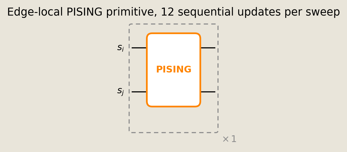
The schematic isolates the edge-local primitive from which the circuit is assembled. The two wires encode the endpoint spins, while the box applies their PISING update. It does not depict a simultaneous 12-edge layer: a sweep is the ordered list of 12 edges printed below, with one matrix applied after another.
The instance is small enough that we never have to guess at a reference. With 8 nodes the exact classical probability vector has only $2^8 = 256$ entries, so we can compute the full distribution, the brute-force optimum, and the exact log-probability scores directly, and every later claim can be checked against an exact number instead of an estimate.
G, edges = random_regular_maxcut(NUM_NODES, DEGREE, seed=GRAPH_SEED)
num_edges = len(edges)
print(f"edge order ({num_edges} sequential updates per sweep): {edges}")
edge order (12 sequential updates per sweep): [(0, 3), (0, 6), (0, 5), (1, 2), (1, 4), (1, 3), (2, 4), (2, 5), (3, 6), (4, 7), (5, 7), (6, 7)]
We brute-force all $2^8$ bitstrings for the exact optimum and how many of them reach it.
cut_values, opt_cut, n_optimal = brute_force_cuts(edges, NUM_NODES)

print(f"graph     : {DEGREE}-regular  N={NUM_NODES}  seed={GRAPH_SEED}")
print(f"edges     : {num_edges}")
print(f"MaxCut    : {opt_cut} / {num_edges}")
print(f"# optimal : {n_optimal} bitstrings out of 2^{NUM_NODES}")
graph     : 3-regular  N=8  seed=7
edges     : 12
MaxCut    : 10 / 12
# optimal : 4 bitstrings out of 2^8
The exact classical probability vector
Both the training gradient and the diagnostic curve begin with the circuit's exact distribution, so we construct that common primitive first.
make_expected_cut returns two pure-jax functions of the couplings. density(J) is the circuit's exact 256-entry classical probability vector, while expected_cut(J) averages the cut over that vector. The core implementation from examples/helpers/_nb09_maxcut.py is:
def make_expected_cut(
    edges: _Edges, num_nodes: int, *, beta: float, dt: float, reps: int
):
    ...
    sim = StateVectorSimulator()
    spins = jnp.asarray(spin_table(num_nodes))
    x0 = jnp.ones(2**num_nodes) / float(2**num_nodes)
    edge_sites = [[int(i), int(j)] for i, j in edges]
    # gate structure is static; trainable couplings J enter through theta pytrees
    circuit = DiscretePCircuit([PISING(sites) for sites in edge_sites], reps=reps)
    edge_i = jnp.asarray([i for i, _ in edge_sites])
    edge_j = jnp.asarray([j for _, j in edge_sites])

    def density(J):
        thetas = [
            jnp.stack([J[e], 0.0, 0.0, jnp.asarray(beta), jnp.asarray(dt)])
            for e in range(len(edge_sites))
        ]
        compiled = sim.build_circuit(circuit, thetas)
        return sim.density(compiled, x0)

    def expected_cut(J):
        rho = density(J)
        edge_products = spins[:, edge_i] * spins[:, edge_j]
        correlations = rho @ edge_products
        return jnp.sum((1.0 - correlations) / 2.0)

    return expected_cut, density
Within each sweep, Discrete applies the 12 PISING gates sequentially in edges order and then repeats the ordered sweep REPS times.
The two returned functions serve different roles. Training samples indices from density and differentiates the corresponding entries of its exact log-probability vector, so the couplings receive gradients only through sampled log probabilities. By contrast, expected_cut does not drive an update; it is evaluated only as an exact simulator diagnostic beside the sampled batch objective.
Before training, we evaluate this diagnostic at the initial couplings. We also compute the mean cut of a uniform random assignment and the brute-force optimum. These values provide the two reference levels against which we will read the training curves.
# Build the exact readout once, then reuse it for all couplings.
expected_cut, density = make_expected_cut(edges, NUM_NODES, beta=BETA, dt=DT, reps=REPS)

J_init = jnp.full((num_edges,), J_INIT)
uniform_mean = float(cut_values.mean())

print(f"expected cut at initialization: {float(expected_cut(J_init)):.2f}")
print(f"uniform baseline (mean cut):    {uniform_mean:.2f}")
print(f"brute-force optimum:            {opt_cut} / {num_edges}")
expected cut at initialization: 6.51
uniform baseline (mean cut):    6.00
brute-force optimum:            10 / 12
Training by REINFORCE
We now run the training loop and compare two curves: the sampled quantity that drives the optimizer and the exact quantity that checks it.
We maximize $\mathbb{E}_{p_\theta}[\mathrm{cut}]$ with a likelihood-based REINFORCE estimator and optax.adam. At each step, the code computes the complete vector density_fn(J), draws NUM_SAMPLES bitstrings from it, and differentiates the selected exact log probabilities. For a batch of $M>1$ bitstrings, with $\bar c$ denoting the same-batch mean cut, the implemented estimator is
$$ \nabla_\theta\,\mathbb{E}_{p_\theta}[\mathrm{cut}] \;\approx\; \frac{1}{M-1}\sum_{m=1}^{M}\bigl(\mathrm{cut}(x_m)-\bar c\bigr)\,\nabla_\theta\log p_\theta(x_m), \qquad x_m\sim p_\theta. $$
Because the samples also determine $\bar c$, simply averaging the centered terms would introduce a finite-batch factor. The code multiplies the centered same-batch surrogate by $M/(M-1)$, which corrects that factor exactly and leaves the estimator unbiased.
The batch-mean cut is the quantity observed by the optimizer. The exact expected cut is computed separately from all 256 probabilities, never supplied to a gradient, and used only to test whether the sampled objective tracks the underlying distribution. Keeping these curves separate lets us compare optimization evidence with an exact diagnostic.
def train_couplings(density_fn, expected_cut_fn, cut_values, num_edges, *,
                    steps, num_samples, lr, key):
    """Train couplings with a finite-batch-corrected REINFORCE estimator.

    Each step differentiates selected entries of the exact full log-probability
    vector returned by ``density_fn``. The exact ``expected_cut_fn`` is evaluated
    only to record a diagnostic trajectory.
    """
    if num_samples < 2:
        raise ValueError("num_samples must be at least 2 for baseline correction")
    cut_values = jnp.asarray(cut_values)
    correction = num_samples / (num_samples - 1)

    def surrogate(J, key):
        logp = jnp.log(density_fn(J))
        idx = jax.random.categorical(key, jax.lax.stop_gradient(logp), shape=(num_samples,))
        cuts = cut_values[idx]
        sampled_mean = jnp.mean(cuts)
        centered = jax.lax.stop_gradient(cuts - sampled_mean)
        loss = -correction * jnp.mean(centered * logp[idx])
        return loss, sampled_mean

    surrogate_value_and_grad = jax.jit(jax.value_and_grad(surrogate, has_aux=True))
    expected_cut_jit = jax.jit(expected_cut_fn)
    optimizer = optax.adam(lr)
    J = jnp.full((num_edges,), J_INIT)
    opt_state = optimizer.init(J)
    expected_hist = [float(expected_cut_jit(J))]
    sampled_hist = []
    for _ in range(steps):
        key, subkey = jax.random.split(key)
        (_loss, sampled_mean), grads = surrogate_value_and_grad(J, subkey)
        updates, opt_state = optimizer.update(grads, opt_state)
        J = optax.apply_updates(J, updates)
        sampled_hist.append(float(sampled_mean))
        expected_hist.append(float(expected_cut_jit(J)))
    return J, expected_hist, sampled_hist
J_star, expected_hist, sampled_hist = train_couplings(
    density, expected_cut, cut_values, num_edges,
    steps=TRAIN_STEPS, num_samples=NUM_SAMPLES, lr=LEARNING_RATE,
    key=jax.random.PRNGKey(TRAIN_SEED),
)
print(f"exact expected-cut diagnostic: {expected_hist[0]:.2f} -> {expected_hist[-1]:.2f}   (optimum {opt_cut})")
print(f"sampled batch objective:       {sampled_hist[0]:.2f} -> {sampled_hist[-1]:.2f}")
print(f"trained couplings: mean {float(J_star.mean()):.2f}, std {float(J_star.std()):.2f}")
assert expected_hist[-1] > expected_hist[0]
fig = plot_training_trajectory(
    expected_hist, sampled_hist, opt=opt_cut, uniform_mean=uniform_mean,
    num_samples=NUM_SAMPLES,
)
savefig(fig, "09_sgnn_training")
exact expected-cut diagnostic: 6.51 -> 9.99   (optimum 10)
sampled batch objective:       6.55 -> 9.99
trained couplings: mean -2.26, std 2.52
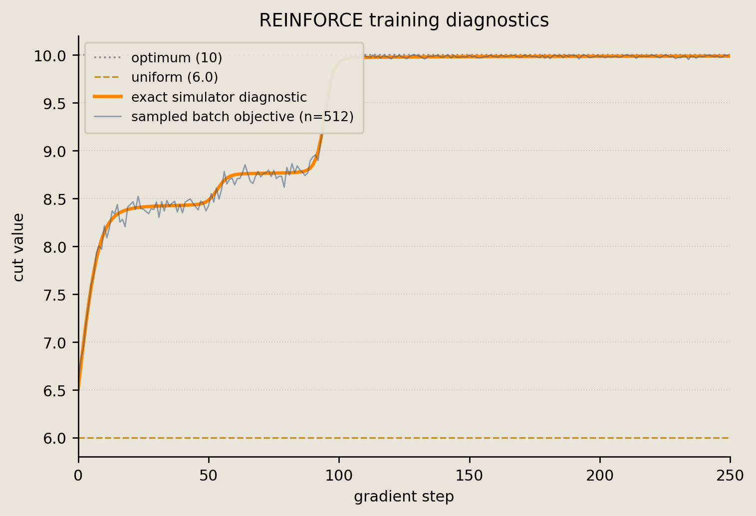
Both curves rise together from about 6.5 to 9.99 against an optimum of 10, which is the agreement we wanted: the sampled objective the optimizer follows tracks the exact expected cut rather than drifting away from it. The exact diagnostic carries one extra point because we evaluate it at the initial couplings before any update, while the sampled batch mean is recorded from the batch drawn at each step.
What the circuit learned
Raising an average says nothing about where the probability went, so we now compare the exact cut distribution of the trained circuit against the uniform baseline.
# Convert exact output distributions into distributions over cut values.
rho_learned = np.asarray(density(J_star))
cut_support = np.arange(num_edges + 1)

uniform_dist = cut_distribution(
    np.full(2**NUM_NODES, 1.0 / 2**NUM_NODES),
    cut_values,
    num_edges,
)
learned_dist = cut_distribution(rho_learned, cut_values, num_edges)
print(f"learned mass on the optimum   : {learned_dist[opt_cut]:.3f}")
print(
    f"learned mass on cut >= {opt_cut - 1}      : {learned_dist[opt_cut - 1:].sum():.3f}"
)

fig = plot_cut_distribution(
    cut_support,
    uniform_dist,
    learned_dist,
    opt=opt_cut,
)
savefig(fig, "09_sgnn_cut_distribution")
learned mass on the optimum   : 0.996
learned mass on cut >= 9      : 0.997
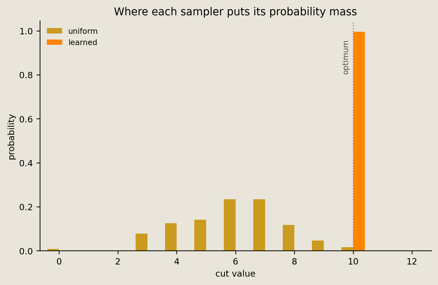
The trained circuit places 0.996 of its probability on the optimum itself and 0.997 within one edge of it, so training concentrated the distribution rather than merely nudging its mean. The uniform baseline stays spread around a mean cut of 6.00, far below the optimum of 10.
The cut distribution identifies the dominant score but not the corresponding partition. We therefore decode the most probable trained bitstring and draw it on the graph, highlighting the edges that cross between its two groups.
# Decode the most likely state index into one bit per graph node.
best_index = int(np.argmax(rho_learned))
partition = np.array(
    [(best_index >> (NUM_NODES - 1 - q)) & 1 for q in range(NUM_NODES)]
)
learned_cut = int(sum(partition[i] != partition[j] for i, j in edges))
print(f"most-probable bitstring cut: {learned_cut} / {num_edges}")

fig = plot_partition(
    G,
    partition,
    learned_cut=learned_cut,
    num_edges=num_edges,
    layout_seed=GRAPH_SEED,
)
savefig(fig, "09_sgnn_graph")
most-probable bitstring cut: 10 / 12
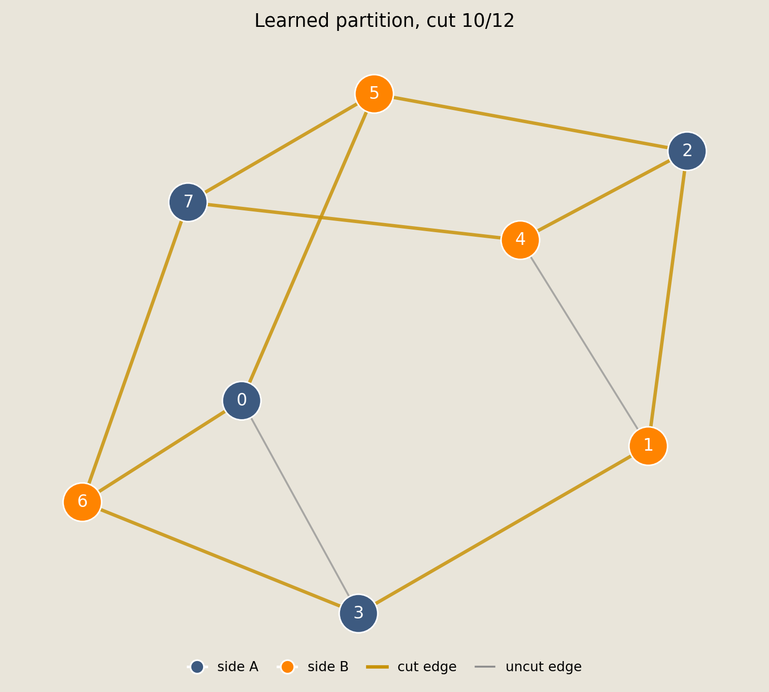
Ten of the 12 edges are gold, which equals the brute-force optimum, so the mode of the trained distribution is an exact MaxCut solution. Gold edges cross the cut, and neutral gray edges join two nodes on the same side.
Verification
Each check below tests one claim the figures rest on against a reference we can compute exactly.
- Every trained
PISINGmatrix still has columns summing to one, which confirms the learned couplings describe a valid stochastic update rather than an arbitrary matrix. - The final exact expected cut exceeds both its value at initialization and the uniform baseline, which establishes that REINFORCE training, and not the circuit's starting point, produced the improvement.
- More than half the trained probability mass sits on cuts within one edge of the optimum, which shows the circuit concentrates on good partitions instead of only shifting its average.
- The most probable trained bitstring attains the brute-force optimum, so the mode of the learned distribution is an exact solution.
- Three further graph seeds (11, 23, and 41) each finish above their own initial and uniform values and reach at least 80% of their brute-force optimum, which shows the result doesn't depend on the single graph drawn with
GRAPH_SEED.
# 1) Each trained PISING edge is column-stochastic.
trained_mats = np.stack([edge_pising_matrix(float(j), beta=BETA, dt=DT) for j in J_star])
np.testing.assert_allclose(trained_mats.sum(axis=-2), 1.0, atol=1e-6)

# 2) REINFORCE training raised the expected cut past the uniform baseline.
assert expected_hist[-1] > expected_hist[0]
assert expected_hist[-1] > uniform_mean

# 3) The trained distribution concentrates on near-optimal cuts.
assert learned_dist[opt_cut - 1:].sum() > 0.5

# 4) The most-probable trained bitstring is an optimal cut.
assert learned_cut == opt_cut
# 5) Validation: print three other seeded graphs and enforce explicit thresholds.
validation_rows = []
for seed in (11, 23, 41):
    G_s, edges_s = random_regular_maxcut(NUM_NODES, DEGREE, seed=seed)
    ec_s, density_s = make_expected_cut(edges_s, NUM_NODES, beta=BETA, dt=DT, reps=REPS)
    cut_values_s, opt_s, _ = brute_force_cuts(edges_s, NUM_NODES)
    initial_s = float(ec_s(jnp.full((len(edges_s),), J_INIT)))
    uniform_s = float(cut_values_s.mean())
    J_s, expected_s, sampled_s = train_couplings(
        density_s, ec_s, cut_values_s, len(edges_s),
        steps=TRAIN_STEPS, num_samples=NUM_SAMPLES, lr=LEARNING_RATE,
        key=jax.random.PRNGKey(seed),
    )
    final_s = float(expected_s[-1])
    validation_rows.append((seed, initial_s, uniform_s, final_s, opt_s))
    assert final_s > initial_s
    assert final_s > uniform_s
    assert final_s >= 0.8 * opt_s
print("seed | initial | uniform | final | optimum | final/optimum")
for seed, initial_s, uniform_s, final_s, opt_s in validation_rows:
    print(f"{seed:4d} | {initial_s:7.3f} | {uniform_s:7.3f} | {final_s:5.3f} | {opt_s:7d} | {final_s / opt_s:13.1%}")
seed | initial | uniform | final | optimum | final/optimum
  11 |   6.512 |   6.000 | 8.759 |      10 |         87.6%
  23 |   6.494 |   6.000 | 8.874 |      10 |         88.7%
  41 |   6.541 |   6.000 | 8.813 |      10 |         88.1%
With the assertions passing, we print the headline numbers.
print("all checks passed")
print(f"  expected cut   {expected_hist[0]:.2f} -> {expected_hist[-1]:.2f}  (optimum {opt_cut})")
print(f"  learned mass on optimum   {learned_dist[opt_cut]:.3f}")
print(f"  uniform / learned : {uniform_mean:.2f} / {expected_hist[-1]:.2f}")
all checks passed
  expected cut   6.75 -> 9.99  (optimum 10)
  learned mass on optimum   0.996
  uniform / learned : 6.00 / 9.99
Conclusion
We built a stochastic graph network for MaxCut with one PISING gate per edge, then trained its couplings with REINFORCE.
- Each sweep applies 12 column-stochastic Glauber updates sequentially in fixed edge-list order, then repeats that sweep 20 times.
- The estimator samples from the exact Torx probability vector and differentiates its selected exact log probabilities. Multiplying the same-batch centered surrogate by $M/(M-1)$ removes its finite-batch bias.
- The training figure keeps the sampled batch objective, which is what the optimizer sees, separate from the exact expected-cut diagnostic, which we evaluate before the first update and so starts at step zero.
- The exact learned distribution concentrates on high-cut partitions, and three additional graph seeds print their initial, uniform, final, optimum, and final-to-optimum values so the result can be judged beyond one graph.
See also:
06_ising_sampling_contrastive_divergence.ipynb, which covers thePISINGGlauber kernel and learning its couplings.04_execution_interface_readouts.ipynb, which covers how the simulators estimate expectations.08_stochastic_convolutional_networks.ipynb, the sibling stochastic-network construction.
References
- Williams, R.J. 1992. Simple statistical gradient-following algorithms for connectionist reinforcement learning. Mach. Learn. 8, 229-256.
- Glauber, R.J. 1963. Time-dependent statistics of the Ising model. J. Math. Phys. 4, 294-307.