
Introduction to Torx factors and directed factor graphs
We define four tutorial factors on Torx factor base classes, call each one directly, then place the same factors in a directed graph and two composite factors. At every level, sampling uses sample(key, inputs, params): the object changes from one probabilistic bit to a graph or composite, but the calling convention does not. Because Tiled and Chain only organize calls to an underlying factor, we also compare them with manual JAX equivalents under the same random keys and require the draws to agree exactly.
Torx can sample objects at several levels: an individual probabilistic factor, a directed graph of factors, or a circuit-shaped graph. We begin with the smallest of these objects, a single probabilistic bit (pbit), and then build upward. The pbit receives a factor of its own, two factors are wired into a Torx directed factor graph, and the resulting hierarchy is related to the parametrised stochastic circuit (PSC) view used elsewhere in the gallery.
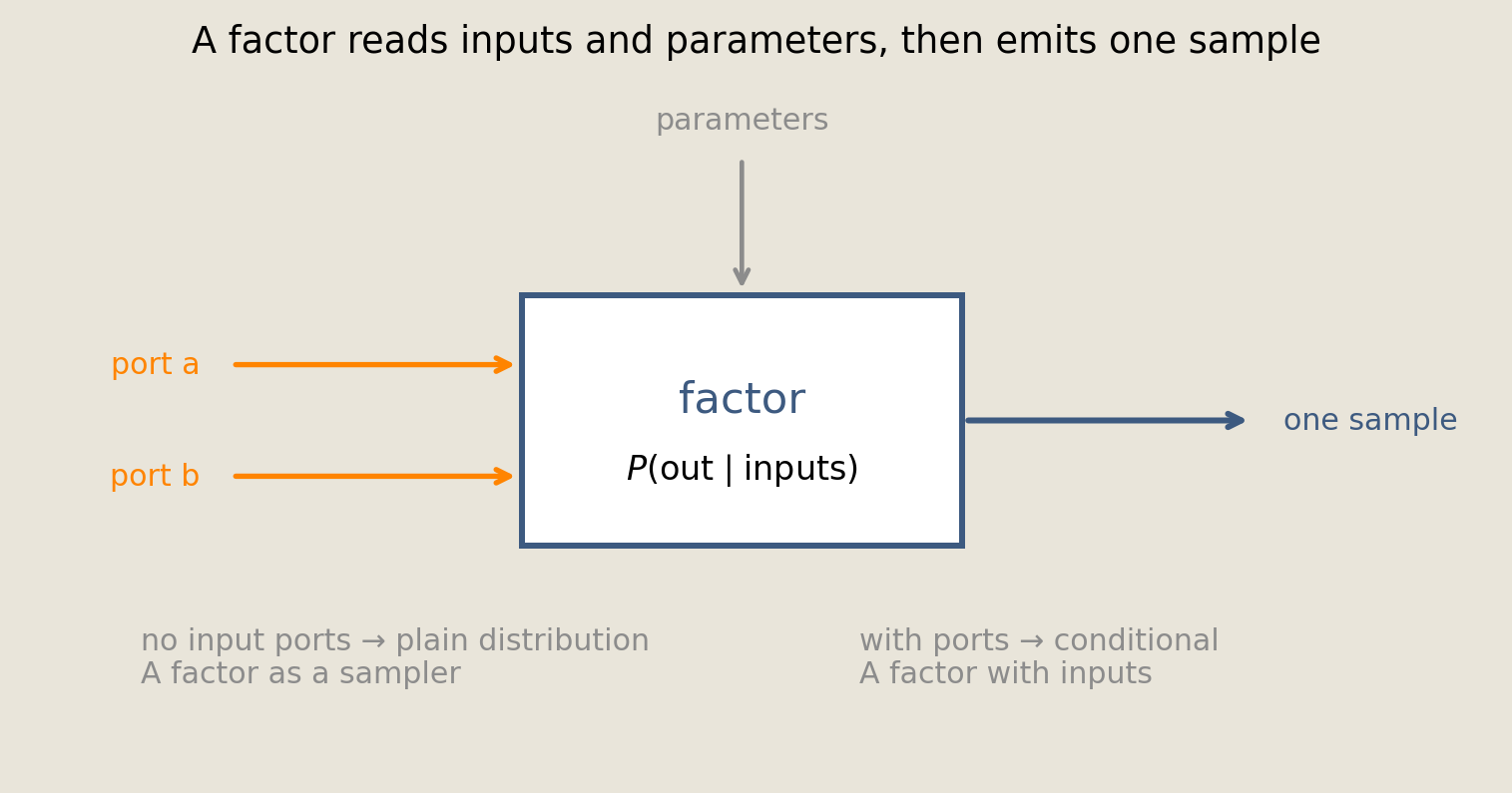
A factor packages one conditional distribution as an object. It reads named inputs and parameters supplied with each call, then returns one stochastic output. The parameters remain outside the object, so the same factor can be reused with different values rather than retaining numbers that may become stale. The four probability laws in this notebook belong to CoinFactor, ConditionalBit, TinyCategorical, and FlipFactor; these are tutorial classes, not Torx library primitives. Torx supplies the base classes, graph, and composites that invoke them.
A directed factor graph wires the output of one factor into the input of another. Because the wiring has no cycles, its nodes can be sampled once in parent-to-child order. Torx gates are also factors through their base classes, so a gate and a bare factor differ in how much placement has already been specified, not in whether they define a probability model. A PSC fixes factors into circuit wiring, whereas a concrete DFG places factors at named Site nodes in an arbitrary DAG.
Term: Torx DFG and conventional factor graph
A Torx directed factor graph is a DAG of conditional samplers, while the conventional factor graph of Kschischang et al. is a bipartite graph of variable and factor nodes. A PSC subclasses Torx Abstract as a circuit-shaped implementation, but it isn't a subclass of the concrete Torx DFG class.
This tutorial develops the factor-side view of the construction introduced from the PSC side in notebook 01. Notebook 16 applies the same composition mechanism to Gibbs sampling on a larger factor graph.
Setup
Before any factor exists we need paths, imports, styling, figure export, and a way to describe a port without allocating an array for it. jax.ShapeDtypeStruct records a port's shape and dtype without allocating data, so we use it to declare the only two port types this notebook needs: BIT describes one integer pbit, and DRIVE one scalar floating-point input.
The examples/helpers modules used here handle paths, style, and plots only, which means none of the probability model is hidden inside them.
from pathlib import Path
import sys

import equinox as eqx
import jax
import jax.numpy as jnp
import numpy as np
ROOT = Path.cwd()
if not (ROOT / "helpers").exists() and (ROOT.parent / "helpers").exists():
    ROOT = ROOT.parent
HELPER_DIR = ROOT / "helpers"
sys.path.insert(0, str(HELPER_DIR))
from _notebook_paths import figure_dir
from _notebook_style import apply_notebook_style, make_savefig
import _plots_sampling as P_samp
import _plots_schematics as P_sch

from torx import (
    AbstractMatrixFactor,
    AbstractReferenceFactor,
    ChainFactor,
    DFG,
    Site,
    TiledFactor,
)
apply_notebook_style()
FIGURE_DIR = figure_dir(ROOT)
SEED = 16


savefig = make_savefig(FIGURE_DIR)
BIT = jax.ShapeDtypeStruct((), jnp.int32)  # one pbit, 0 or 1
DRIVE = jax.ShapeDtypeStruct((), jnp.float32)  # a continuous value on an input port
A tutorial factor as a sampler
We begin with a factor that has no inputs, so its sampling behavior can be examined before any graph wiring is introduced. The notebook-defined CoinFactor subclasses Torx Abstract and declares no input ports, making it a distribution over one pbit.
The call coin.sample(k, {}, coin_params) exposes the three parts of the sampling convention. k supplies the random key, the empty dictionary records that this factor has no inputs, and coin_params supplies the external parameter dictionary. The custom sample method calls jax.random.bernoulli directly to draw 1 with probability $\sigma(b)$.
class CoinFactor(AbstractReferenceFactor):
    """P(coin) with no inputs: one pbit drawn 1 with probability sigmoid(bias)."""

    input_ports: dict[str, jax.ShapeDtypeStruct] = eqx.field(static=True)
    output_spec: jax.ShapeDtypeStruct = eqx.field(static=True)

    def __init__(self):
        self.input_ports = {}
        self.output_spec = BIT

    def init_params(self, key):
        return {"bias": jnp.array(0.4)}

    def sample(self, key, inputs, params, info=None, site_info=None, return_aux=False):
        out = jax.random.bernoulli(key, jax.nn.sigmoid(params["bias"])).astype(jnp.int32)
        return (out, None) if return_aux else out
coin = CoinFactor()
coin_params = coin.init_params(jax.random.key(SEED))
keys = jax.random.split(jax.random.key(SEED + 1), 20_000)
# Many independent keys give a stable Monte Carlo estimate of the pbit mean.
coin_draws = jax.vmap(lambda k: coin.sample(k, {}, coin_params))(keys)
coin_mean = float(coin_draws.mean())
coin_target = float(jax.nn.sigmoid(coin_params["bias"]))
print(f"sampled P(coin=1) = {coin_mean:.3f}   target sigmoid(b) = {coin_target:.3f}")
sampled P(coin=1) = 0.601 target sigmoid(b) = 0.599
Across 20,000 independent keys, the sampled frequency of 1 is 0.601, compared with the target $\sigma(b)=0.599$. Their difference is well within the tolerance of 0.02 asserted at the end of the notebook, so this sample is consistent with the distribution declared by CoinFactor.
A tutorial factor with inputs
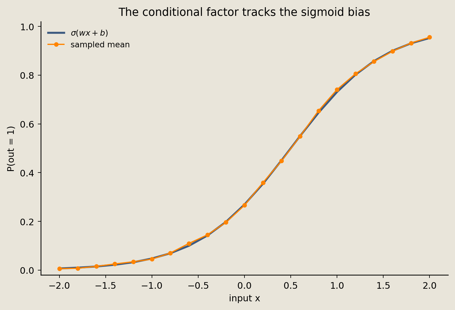
A graph can route information into a factor only if that factor declares an input port. The notebook-defined ConditionalBit therefore keeps the same Torx base contract as CoinFactor but adds one named input. Its probability law is
$$ P(\text{out}=1 \mid x)=\sigma(wx+b). $$
We evaluate this law at 21 drive values by mapping calls to ConditionalBit.sample over independent JAX keys. In the figure, the sampled means are plotted against the corresponding sigmoid curve. Agreement across the full sweep, rather than only near its midpoint, tests whether the drive input enters the bias with the declared weight.
class ConditionalBit(AbstractReferenceFactor):
    """P(out | drive): one pbit whose bias is shifted by an input."""

    input_ports: dict[str, jax.ShapeDtypeStruct] = eqx.field(static=True)
    output_spec: jax.ShapeDtypeStruct = eqx.field(static=True)

    def __init__(self):
        self.input_ports = {"drive": DRIVE}
        self.output_spec = BIT

    def init_params(self, key):
        return {"w": jnp.array(2.0), "b": jnp.array(-1.0)}

    def sample(self, key, inputs, params, info=None, site_info=None, return_aux=False):
        gamma = params["w"] * inputs["drive"] + params["b"]
        out = jax.random.bernoulli(key, jax.nn.sigmoid(gamma)).astype(jnp.int32)
        return (out, None) if return_aux else out
cond = ConditionalBit()
cond_params = cond.init_params(jax.random.key(SEED + 2))
xs = jnp.linspace(-2.0, 2.0, 21)
N_SWEEP = 8_000
@eqx.filter_jit
def sweep_conditional(xs, params, key):
    # (len(xs), N_SWEEP) keys: nested vmap over input points and samples,
    # one compile and no per-point host sync, then mean over the sample axis.
    """Mean conditional sample at each drive value in `xs`."""
    keys = jax.random.split(key, (xs.shape[0], N_SWEEP))

    def at_x(x, x_keys):
        draws = jax.vmap(lambda k: cond.sample(k, {"drive": x}, params))(x_keys)
        return draws.mean()

    return jax.vmap(at_x)(xs, keys)


sampled = np.asarray(sweep_conditional(xs, cond_params, jax.random.key(SEED + 3)))
exact_curve = np.asarray(jax.nn.sigmoid(cond_params["w"] * xs + cond_params["b"]))
fig = P_samp.plot_conditional_sweep(np.asarray(xs), sampled, exact_curve)
savefig(fig, "15_conditional_sweep")
Wiring tutorial factors into a Torx directed factor graph
A Torx Site records how an individual factor participates in a graph. It names the factor's parents, routes parent outputs to input ports, and selects a parameter slice with param_key. Torx DFG then visits the sites in topological order—parents before children—so the entire directed graph can be sampled in one pass (Pearl 1988).
The tables and figures below distinguish the objects that define probability laws from those that execute, compose, or display them:
| Label used below | Owner |
|---|---|
| Torx primitive | Abstract, Abstract, Site, DFG, Tiled, Chain |
| Tutorial factor | the four notebook-defined classes and their probability formulas |
| Notebook JAX | batching, compilation, estimates, and checks |
| Plot helper | presentation only |
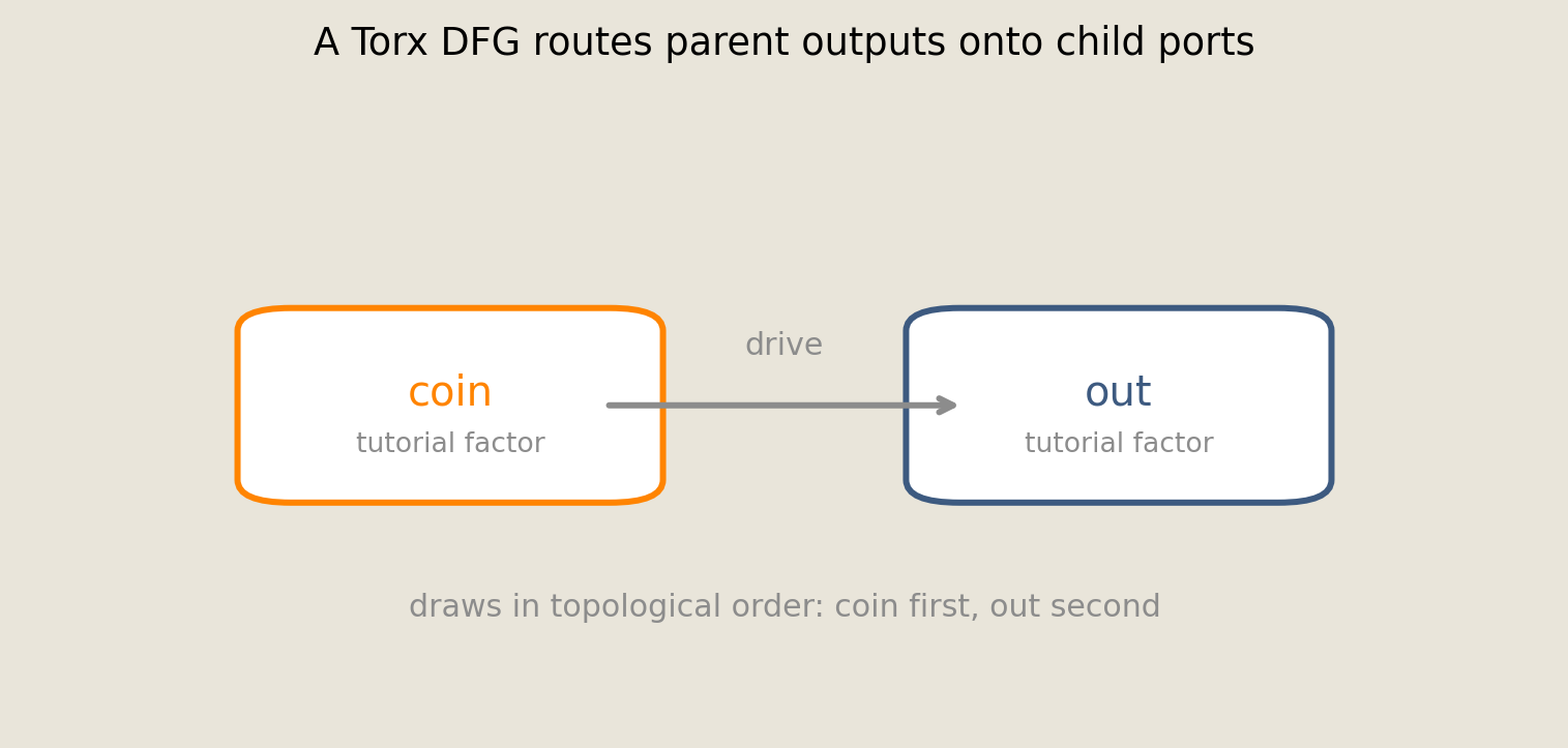
The concrete graph contains two notebook-defined factors. coin is sampled first. The notebook function to_drive then casts its integer output to the floating-point value required by the drive port of out. The graph retains the sample(key, inputs, params) contract, so graph.sample(key, {}, dfg_params) has the same calling convention as the single factor.
For the fixed tutorial parameters, one path through the graph has these values and owners:
| Step | Value | Owner |
|---|---|---|
CoinFactor.sample |
coin = 1 |
tutorial factor called by Torx DFG |
to_drive |
{"drive": 1.0} |
notebook routing function |
ConditionalBit score |
$2(1)-1=1$ | tutorial formula |
| child probability | $P(\mathrm{out}=1)=\sigma(1)=0.731$ | tutorial factor called by Torx DFG |
The factor-anatomy diagram that follows isolates the common boundary: named inputs and external parameters enter a factor, and one sample leaves. Site adds the graph routing around that boundary.
fig = P_sch.plot_factor_anatomy()
savefig(fig, "15_factor_anatomy")
def to_drive(outs):
    """Port the parent bit into the child's continuous drive input."""
    return {"drive": outs[0].astype(jnp.float32)}
sites = (
    # parentless coin: empty porting tuple, no parent outputs to route
    Site("coin", CoinFactor(), (), (), "src", info_key=None, site_info=None),
    Site(
        "out",
        ConditionalBit(),
        ("coin",),
        to_drive,
        "cond",
        info_key=None,
        site_info=None,
    ),
)
graph = DFG(sites, {}, "out")
# init_params walks the sites and returns one param slice per distinct param_key
dfg_params = graph.init_params(jax.random.key(SEED + 4))
one_draw = graph.sample(jax.random.key(SEED + 6), {}, dfg_params)
print(f"one DFG output draw: {int(one_draw)}")

keys = jax.random.split(jax.random.key(SEED + 7), 60_000)
@eqx.filter_jit
def sample_dfg_many(keys, params):
    """Draw one graph sample per key, batched under jit."""
    return jax.vmap(lambda k: graph.sample(k, {}, params))(keys)


dfg_out = sample_dfg_many(keys, dfg_params)
# Marginalize over the hidden coin by hand to check the graph sampler.
p_coin = float(jax.nn.sigmoid(dfg_params["src"]["bias"]))
w, b = dfg_params["cond"]["w"], dfg_params["cond"]["b"]
p_out_g0 = float(jax.nn.sigmoid(w * 0 + b))
p_out_g1 = float(jax.nn.sigmoid(w * 1 + b))
p_out_exact = (1 - p_coin) * p_out_g0 + p_coin * p_out_g1
p_out_emp = float(dfg_out.mean())
print(f"hand-computed P(out=1) = {p_out_exact:.3f}   sampled = {p_out_emp:.3f}")
one DFG output draw: 1
hand-computed P(out=1) = 0.546 sampled = 0.549
Across 60,000 graph draws, the sampled mean of out is 0.549; marginalizing the hidden coin by hand gives 0.546. This agreement is consistent with the joint distribution defined by the two tutorial factors and checks the routing and parent-first execution used in this example. The schematic below encodes that execution path: coin is the parent, to_drive converts its output for the child's input port, and out is sampled second. The schematic shows the dependency structure, while the two means provide the numerical comparison.
fig = P_sch.plot_two_node_dfg()
savefig(fig, "15_two_node_dfg")
Exact probabilities as an opt-in capability
Every factor implements sampling, but only some factors can report their distribution in closed form. Torx represents this as an additional capability rather than a requirement on all factors. The notebook-defined TinyCategorical subclasses Torx Abstract, retaining the common sampling interface while adding get_log_probability_matrix.
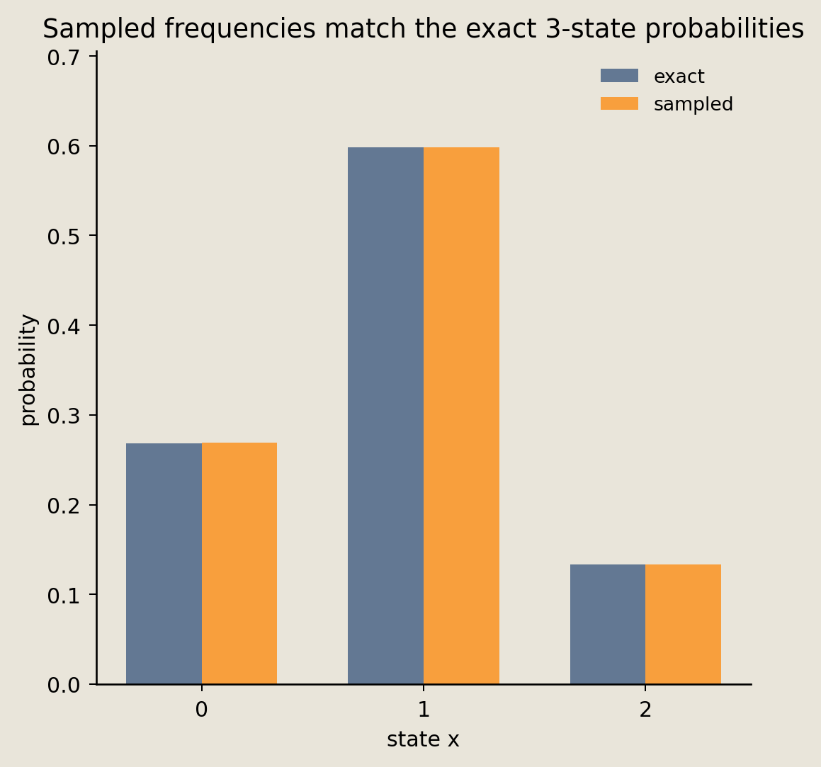
For a matrix factor, rows enumerate input configurations and columns enumerate output configurations; input_states and output_states define those orders. TinyCategorical has no inputs, so its matrix contains one row for the empty input configuration and three columns ordered as x = 0, 1, 2. Each entry is a normalized log probability. Exponentiating the row therefore produces probabilities that sum to one.
The call cat.sample(k, {}, cat_params) still uses the same three arguments as the earlier factors. Its sample is a dictionary keyed by output name, so the categorical value is read with ["x"].
class TinyCategorical(AbstractMatrixFactor):
    """A finite 3-state pdit, no inputs, that also reports exact probabilities."""

    input_states: dict[str, jax.Array]
    output_states: dict[str, jax.Array]

    def __init__(self):
        self.input_states = {}
        self.output_states = {"x": jnp.arange(3)}

    def init_params(self, key):
        return {"logits": jnp.array([0.2, 1.0, -0.5])}

    def sample(self, key, inputs, params, info=None, site_info=None, return_aux=False):
        row = self.get_log_probability_matrix(params, info, site_info)[0]
        out = self.get_nth_output_state(jax.random.categorical(key, row))
        return (out, None) if return_aux else out

    def get_log_probability_matrix(self, params, info=None, site_info=None):
        logits = params["logits"]
        return (logits - jax.scipy.special.logsumexp(logits))[None, :]
cat = TinyCategorical()
cat_params = cat.init_params(jax.random.key(SEED + 8))
exact_p = np.asarray(jnp.exp(cat.get_log_probability_matrix(cat_params))[0])
print("exact probabilities:")
for s, p in enumerate(exact_p):
    print(f"  P(x = {s}) = {p:.3f}")
print(f"  sum        = {exact_p.sum():.3f}")

keys = jax.random.split(jax.random.key(SEED + 18), 50_000)
cat_draws = jax.vmap(lambda k: cat.sample(k, {}, cat_params))(keys)["x"]
# Compare the exact row with frequencies from many categorical draws.
emp_p = np.asarray(jax.vmap(lambda s: jnp.mean(cat_draws == s))(jnp.arange(3)))
exact probabilities:
  P(x = 0) = 0.269
  P(x = 1) = 0.598
  P(x = 2) = 0.133
  sum        = 1.000
The frequencies from 50,000 draws reproduce the exact row of 0.269, 0.598, and 0.133 to within the tolerance of 0.02 asserted at the end, so the opt-in probability table and the sampling contract describe one distribution rather than two that merely resemble each other. The bar chart below plots the two side by side, one pair of bars per state.
fig = P_samp.plot_categorical_parity(exact_p, emp_p)
savefig(fig, "15_categorical_parity")
Torx composites around a tutorial transition
We now consider two forms of repeated sampling: applying one factor to several inputs in parallel, and applying it repeatedly while feeding each output into the next step. The notebook-defined FlipFactor supplies the transition law for both constructions. Torx Tiled evaluates eight weight-tied copies in parallel, whereas Torx Chain evaluates five weight-tied steps and feeds each output back through the state port. Here, weight tying means that every copy or step receives the same parameter slice rather than a separate one.
class FlipFactor(AbstractReferenceFactor):
    """P(next | state): a 2-state telegraph step. Input port and output are both pbits."""

    input_ports: dict[str, jax.ShapeDtypeStruct] = eqx.field(static=True)
    output_spec: jax.ShapeDtypeStruct = eqx.field(static=True)

    def __init__(self):
        self.input_ports = {"state": BIT}  # same dtype as the output: int to int
        self.output_spec = BIT

    def init_params(self, key):
        return {"w": jnp.array(1.5), "b": jnp.array(0.0)}

    def sample(self, key, inputs, params, info=None, site_info=None, return_aux=False):
        gamma = params["b"] + params["w"] * (2 * inputs["state"] - 1)
        out = jax.random.bernoulli(key, jax.nn.sigmoid(gamma)).astype(jnp.int32)
        return (out, None) if return_aux else out
flip = FlipFactor()
flip_params = flip.init_params(jax.random.key(SEED + 9))

# Torx TiledFactor: 8 tied copies of the notebook-defined transition.
tiled = TiledFactor(flip, n_tiles=8, weight_tied=True)
tiled_out = tiled.sample(
    jax.random.key(SEED + 10), {"state": jnp.zeros(8, jnp.int32)}, flip_params
)

# Torx ChainFactor: 5 tied steps with output fed back to state.
chain = ChainFactor(flip, n_steps=5, feedback_porting_fn="state", weight_tied=True)
chain_out = chain.sample(
    jax.random.key(SEED + 11), {"state": jnp.array(0, jnp.int32)}, flip_params
)
print(f"tiled 8 parallel draws: {np.asarray(tiled_out)}")
print(f"chain after 5 steps:    {int(chain_out)}")
tiled 8 parallel draws: [1 0 0 0 1 0 1 0]
chain after 5 steps:    1
Both composites reuse the same FlipFactor and the same parameter slice. In Tiled, that slice is shared across eight parallel draws. In Chain, the output state is fed through the same tied transition five times, and the composite returns the state after the fifth step.
The corresponding calls retain the factor convention. tiled.sample(key, {"state": states}, flip_params) receives eight states, while chain.sample(key, {"state": state}, flip_params) receives the initial scalar state. Their input objects reflect different computations, but both calls still supply a random key, named inputs, and external parameters in the same order as flip.sample.
One sampling interface at every level
Across the examples above, the sampled object and the shape of its inputs change, but every call retains the form sample(key, inputs, params). CoinFactor, ConditionalBit, and TinyCategorical sample individual probability laws. DFG adds parent routing and topological execution, while Tiled and Chain add parallel or repeated calls around another factor without changing the boundary.
A PSC also specializes Abstract, but fixes factors into circuit wiring rather than instantiating the concrete DFG class for an arbitrary DAG. Notebook 01 develops that PSC implementation, while notebook 16 uses factor composition for Gibbs sampling.
Verification
We now compare each Monte Carlo estimate with its corresponding exact value. These checks use finite-sample tolerances because independent draws need not match their expectations exactly.
The composites permit a stricter comparison. Since they reorganize calls to FlipFactor without changing its transition law, we supply identical random keys to each composite and to a manual JAX construction. Tiled must then match a manual vmap over the same split keys, and Chain must match a manual loop that feeds each output back under the same sequence of split keys. A final check compares a one-step chain with the bare factor.
COIN_MEAN_TOL = 0.02  # ~5 sigma at N=20000
COND_SWEEP_TOL = 0.03  # finite-sample
DFG_MEAN_TOL = 0.02  # finite-sample
CAT_FREQ_TOL = 0.02  # finite-sample
CHAIN_MEAN_TOL = 0.03  # finite-sample
assert abs(coin_mean - coin_target) < COIN_MEAN_TOL, (coin_mean, coin_target)
assert np.max(np.abs(sampled - exact_curve)) < COND_SWEEP_TOL
assert abs(p_out_emp - p_out_exact) < DFG_MEAN_TOL, (p_out_emp, p_out_exact)
assert abs(exact_p.sum() - 1.0) < 1e-5
assert np.max(np.abs(emp_p - exact_p)) < CAT_FREQ_TOL, (emp_p, exact_p)
# deterministic same-key check: TiledFactor == manual vmap over split keys
tiled_ref = jax.vmap(
    lambda k: flip.sample(k, {"state": jnp.array(0, jnp.int32)}, flip_params)
)(jax.random.split(jax.random.key(SEED + 10), 8))
np.testing.assert_array_equal(np.asarray(tiled_out), np.asarray(tiled_ref))
# deterministic same-key check: ChainFactor(n_steps=5) == manual feedback scan
manual_state = jnp.array(0, jnp.int32)
for step_key in jax.random.split(jax.random.key(SEED + 11), 5):
    manual_state = flip.sample(step_key, {"state": manual_state}, flip_params)
assert int(chain_out) == int(manual_state), (int(chain_out), int(manual_state))
chain1 = ChainFactor(flip, n_steps=1, feedback_porting_fn="state", weight_tied=True)
seed_state = jnp.array(0, jnp.int32)
chain_keys = jax.random.split(jax.random.key(SEED + 12), 20_000)
flip_keys = jax.random.split(jax.random.key(SEED + 13), 20_000)
chain1_draws = jax.vmap(lambda k: chain1.sample(k, {"state": seed_state}, flip_params))(
    chain_keys
)
flip_draws = jax.vmap(lambda k: flip.sample(k, {"state": seed_state}, flip_params))(
    flip_keys
)
assert abs(float(chain1_draws.mean() - flip_draws.mean())) < CHAIN_MEAN_TOL
# ChainFactor splits step keys internally.
chain_key = jax.random.key(SEED + 12)
one_step = chain1.sample(chain_key, {"state": seed_state}, flip_params)
single = flip.sample(
    jax.random.split(chain_key, 1)[0], {"state": seed_state}, flip_params
)
assert int(one_step) == int(single), (one_step, single)
print("all checks passed")
all checks passed
Conclusion
We defined four tutorial probability laws and composed them with Torx's graph and factor abstractions. The custom classes contain the probability formulas and call JAX random primitives directly; Torx supplies the factor contracts, Site, DFG, Tiled, and Chain that compose them.
A single factor, a directed graph, and a composite factor are all invoked through sample(key, inputs, params). Site and DFG add routing and parent-first execution, while Tiled and Chain apply one factor in parallel or repeatedly with feedback. A Torx DFG is a directed sampler DAG, distinct from a conventional bipartite factor graph. A PSC specializes Abstract as a circuit-shaped implementation and is not a subclass of concrete DFG.
For the circuit-shaped construction, return to notebook 01. For the larger Ising model built through factor composition, continue to notebook 16.
References
- Kschischang, F.R., Frey, B.J., Loeliger, H.A. 2001. Factor graphs and the sum-product algorithm. IEEE Transactions on Information Theory 47(2), 498-519.
- Pearl, J. 1988. Probabilistic Reasoning in Intelligent Systems. Morgan Kaufmann. Directed acyclic graphical models and ancestral generation.