
Gaussian-categorical clustering as a Boltzmann machine
A Gaussian mixture can be read as one joint energy over a continuous visible vector and a categorical hidden unit. Fixing the visible vector gives a softmax over cluster labels—the responsibilities—while fixing the label gives the corresponding Gaussian. We use these two conditionals to recover clusters with hard assignments above 99%, and then alternate them in a Gibbs chain whose occupancy relaxes to the mixture weights.
Many clustering problems combine a continuous observation with an unobserved choice of component. How can one model support both assigning an observed point to a cluster and generating a new point from a chosen cluster? In this tutorial, we answer that question by writing a Gaussian mixture as one energy function and reading it as a Boltzmann machine (Ackley et al. 1985).
The model has two variables. A Gaussian visible vector $v$ represents the observation, and a categorical hidden state $h$ selects its component. In Torx, these are carried by the continuous pmode and categorical pdit data primitives. The $K$-state pdit makes $h$ one-hot, so exactly one cluster is active at a time.
Term: pmode and pdit
A pmode is continuous-valued, while a pdit stores one of $K$ discrete states. The categorical state $k$ corresponds to the one-hot vector $e_k$ in the derivation.
We first derive the joint Boltzmann kernel $p(v,h)\propto e^{-E(v,h)}$. We then execute the model through its two conditionals, which is why the code carries $(\mu_k,\Sigma_k,\pi_k)$ rather than constructing a single joint Torx energy object.
The main steps are:
- write the mixture as one joint energy $E(v,h)$ and derive the cluster probabilities,
- draw labels with NumPy and conditional Gaussian samples with Torx, and
- recover the clusters in JAX, then run a handwritten JAX block Gibbs loop, which redraws one whole block of variables from its conditional while the other block is held fixed.
What runs where?
- NumPy draws mixture labels, counts, and the final shuffle.
- Torx
HybridSampleSimulatorandMixturedraw $v\mid h=k$.Gaussian Gate - JAX computes the Gaussian-mixture responsibilities and the hard assignments taken from them.
- Notebook JAX code implements both Gibbs conditionals directly from the analytic formulas.
This tutorial assumes familiarity with Gaussian mixtures and basic Boltzmann machines. The code uses JAX, NumPy, Matplotlib, and Torx.
Setup
First we import the numerical, plotting, and Torx dependencies used throughout the tutorial. Path and style setup live in examples/helpers/_notebook_paths.py and examples/helpers/_notebook_style.py. The analytic density helper is examples/helpers/_affine_gaussian.py, and figure encodings live in examples/helpers/_plots_fields.py, examples/helpers/_plots_sampling.py, and examples/helpers/_plots_schematics.py, which keeps the modelling cells below short.
from pathlib import Path
import sys
import equinox as eqx
import jax
import jax.numpy as jnp
import numpy as np

ROOT = Path.cwd()
# Allow the notebook to run from the repo root or from the notebooks directory.
if not (ROOT / "helpers").exists() and (ROOT.parent / "helpers").exists():
    ROOT = ROOT.parent
HELPER_DIR = ROOT / "helpers"
sys.path.insert(0, str(HELPER_DIR))
from _notebook_paths import figure_dir
from _notebook_style import apply_notebook_style, make_savefig
from _affine_gaussian import mixture_density
import _plots_fields as P_fld
import _plots_sampling as P_samp
import _plots_schematics as P_sch
from torx.psc import (
    HybridPCircuit,
    MixtureGaussianGate,
)
apply_notebook_style()
FIGURE_DIR = figure_dir(ROOT)
SEED = 123
savefig = make_savefig(FIGURE_DIR)
One energy for a visible vector and a one-hot hidden
A Gaussian mixture is usually introduced as a weighted sum of component densities. To express the same model as a Boltzmann machine, we introduce a one-hot hidden state $h$ that selects one component. For diagonal component variances, the energy used by the code is
$$ E(v,h)=\sum_k h_k\left[\frac{1}{2}\sum_i\frac{(v_i-\mu_{ki})^2}{\sigma_{ki}^2}+\frac{1}{2}\sum_i\log\sigma_{ki}^2-\log\pi_k\right],\qquad p(v,h)\propto e^{-E(v,h)}. $$
The $k$-independent Gaussian normalizer is omitted because it cancels in every comparison across clusters below. The hidden state satisfies
$$ \sum_k h_k=1,\qquad h_k\in\{0,1\}, $$
so $h$ must be one of the $K$ basis states $e_k$. This single energy therefore contains both the continuous observation and the categorical component choice.
How does this mixture energy relate to the usual visible-hidden coupling of a Boltzmann machine? When the components share $\sigma_i$, we can rewrite it as
$$ E(v,h)=\sum_i\frac{(v_i-a_i)^2}{2\sigma_i^2}-\sum_k c_k h_k-\sum_{i,k}\frac{v_i}{\sigma_i}W_{ik}h_k+\text{constant}, $$
with
$$ \mu_k=a+\operatorname{diag}(\sigma)W_{:k},\qquad c_k=\log\pi_k-a^\top\operatorname{diag}(\sigma)^{-1}W_{:k}-\frac{1}{2}\lVert W_{:k}\rVert^2, $$
up to one $k$-independent additive constant. Completing the square contributes the last two terms in the expression for $c_k$, so the bias $c_k$ alone is not the log mixture weight. The code does not need $W$ because it works directly with $(\mu_k,\Sigma_k,\pi_k)$, but the reparameterization shows that the Gaussian mixture has the standard linear visible-hidden coupling.
One modeling choice remains: how should we enforce the one-hot state? A single $K$-state pdit imposes the constraint structurally by representing only the $K$ valid choices. Alternatively, a penalty over $K$ binary units can make the one-hot configurations the ground states. We use the structural representation first, then return to the energetic construction at the end to compare an exact categorical constraint with a winner-take-all penalty of finite strength.
We can now read the energy in two directions. Holding $v$ fixed gives a softmax across the one-hot states, while holding $h=e_k$ fixed gives the Gaussian for component $k$. We begin with three well-separated cluster means, a shared variance, and unequal mixture weights.
K = 3
# Three visible means arranged so the clusters are easy to inspect visually.
cluster_means = jnp.array([[0.0, 3.0], [-2.6, -1.5], [2.6, -1.5]], dtype=jnp.float32)
cluster_vars = jnp.full((K, 2), 0.45, dtype=jnp.float32)
pi = jnp.array([0.40, 0.35, 0.25], dtype=jnp.float32)
log_vars = jnp.log(cluster_vars)
cluster_covs = np.stack([np.diag(np.asarray(cluster_vars[k])) for k in range(K)])

print(f"K={K} clusters")
print(f"means: {np.asarray(cluster_means).round(2).tolist()}")
print(f"diagonal variances: {np.asarray(cluster_vars[0]).round(2).tolist()}")
print(f"mixture weights: {np.asarray(pi).round(2).tolist()}")
K=3 clusters
means: [[0.0, 3.0], [-2.5999999046325684, -1.5], [2.5999999046325684, -1.5]]
diagonal variances: [0.44999998807907104, 0.44999998807907104]
mixture weights: [0.4000000059604645, 0.3499999940395355, 0.25]
As a quick check, we confirm that the mixture weights in pi sum to one.
np.testing.assert_allclose(float(pi.sum()), 1.0, atol=1e-6)
Before specializing either conditional, we look at the factor graph of this energy, because it shows that inference and generation are two readings of one object rather than two separate models.
savefig(P_sch.energy_factor_graph(K), "14_energy_factor_graph")
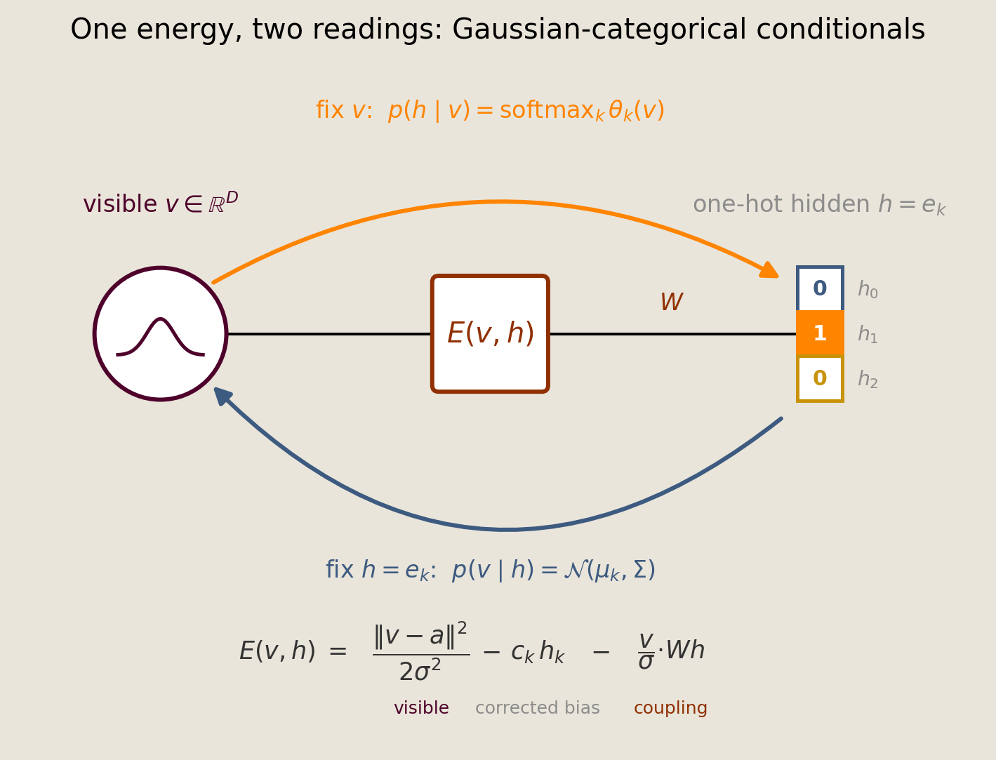
Both directions run through the same factor: fixing $v$ gives the cluster probabilities, and fixing $h=e_k$ gives the Gaussian for cluster $k$.
The softmax emerges
First, fix the visible vector $v$. Because the hidden state can take only one of the basis states $e_k$, the joint energy leaves one score for each component. Normalizing their exponentials gives the categorical conditional
$$ p(h=e_k\mid v)=\operatorname{softmax}_k(\theta(v)),\qquad \theta_k(v)=\log\pi_k-\frac{1}{2}\sum_i\frac{(v_i-\mu_{ki})^2}{\sigma_{ki}^2}-\frac{1}{2}\sum_i\log\sigma_{ki}^2. $$
These probabilities are the Gaussian-mixture responsibilities. The recovery section implements the same score in cluster_logits. With shared covariance and the linear-coupling parameterization above, it can also be written as $\theta_k(v)=c_k+\sum_i(v_i/\sigma_i)W_{ik}$ plus a $k$-independent term, using the corrected $c_k$.
Term: responsibility
A Gaussian-mixture responsibility is the posterior probability $p(h=e_k\mid v)$ that component $k$ generated a point, as in the mixture-model treatment of Dempster et al. 1977.
The form of this conditional follows from the hidden representation: a single bias pbit gives a sigmoid, whereas the one-hot pdit used here gives a softmax. We next obtain the matching continuous conditional and implement it with Mixture.
The Gaussian conditional and the gate
Now fix $h=e_k$. Only the quadratic energy for component $k$ remains, so the conditional over the visible vector is Gaussian:
$$ p(v\mid h=e_k)=\mathcal{N}(v\mid\mu_k,\Sigma_k),\qquad p(v)=\sum_k \pi_k\,\mathcal{N}(v\mid\mu_k,\Sigma_k). $$
The implementation uses $(\mu_k,\Sigma_k,\pi_k)$ in both this conditional and cluster_logits, keeping the generative and inferential readings tied to the same parameters. For shared covariance, $\mu_k=a+\mathrm{diag}(\sigma)W_{:k}$ connects them to the linear-coupling form above.
This is the conditional that Torx executes. Mixture realizes $p(v\mid h=e_k)$, while one pdit stores the cluster index $k\in\{0,1,2\}$ directly. We construct the gate and wrap it in a Hybrid named gen; the circuit infers and preserves the discrete control wire, so a seeded cluster label passes through unchanged.
mog_theta = {"means": cluster_means, "log_vars": log_vars}
# The MixtureGaussianGate is structure only; its means and log-variances live
# in the separate `thetas` list aligned with the circuit gates.
gate = MixtureGaussianGate(sites=(0, 0), dims=(2,), num_components=K)
gen = HybridPCircuit([gate])
thetas = [mog_theta]
We draw the circuit to identify the discrete control and continuous output used by this conditional sampler.
savefig(P_sch.cluster_gate_circuit(), "14_cluster_gate_circuit")
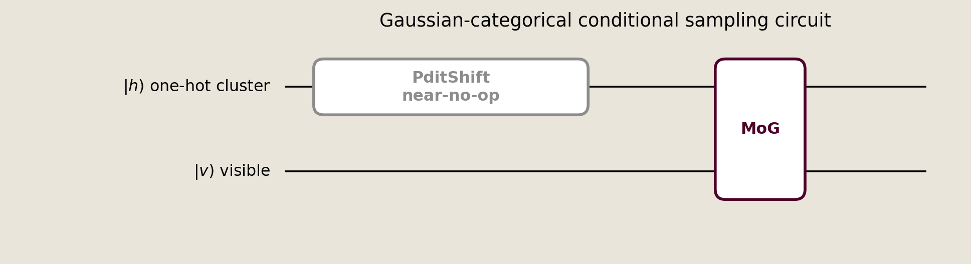
The whole Gaussian mixture is one hybrid gate: the categorical input passes through the near-no-op registration gate, then selects which Gaussian the continuous output comes from.
Generating the clusters
To have something to cluster, we generate a labeled data set whose ground truth we know, splitting the work between two libraries. NumPy draws the component counts from $\pi$ and later shuffles the labeled blocks, and for each NumPy label $k$, Torx seeds the discrete state so that Mixture draws $v\sim\mathcal{N}(\mu_k,\Sigma_k)$.
A multinomial split sets the number of conditional samples requested from each cluster.
N_DATA = 9_000
rng_counts = np.random.default_rng(SEED)
counts = rng_counts.multinomial(N_DATA, np.asarray(pi))
def sample_labeled_mixture(circuit, params, counts):
    """Draw labeled visible samples for each requested cluster count."""
    point_blocks, label_blocks = [], []
    for k, count in enumerate(counts):
        # Seed the pdit to a cluster label, then draw the matching Gaussian block.
        s = circuit.sample_multiple(
            jax.random.key(SEED + 10 + k),
            {"discrete": jnp.array([k], dtype=jnp.int32), "continuous": jnp.zeros(2)},
            params,
            n_samples=int(counts.max()),
        )
        point_blocks.append(np.asarray(s["continuous"])[:count])
        label_blocks.append(np.full(count, k, dtype=np.int32))

    points = np.concatenate(point_blocks, axis=0)
    true_labels = np.concatenate(label_blocks, axis=0)
    # Shuffle the labeled blocks so the data look like a single mixed sample.
    order = np.random.default_rng(SEED + 1).permutation(int(counts.sum()))
    return points[order], true_labels[order]
With the per-cluster counts fixed, we draw the labeled samples directly from gen.
points, true_labels = sample_labeled_mixture(gen, thetas, counts)

sample_props = np.bincount(true_labels, minlength=K) / N_DATA
print(f"counts: {counts.tolist()}  proportions: {sample_props.round(3).tolist()}")
counts: [3686, 3091, 2223] proportions: [0.41, 0.343, 0.247]
Before looking at any figure, we compute the sampled per-cluster moments, because they are the cheapest way to confirm that each block of Torx draws really came from the component we seeded.
cluster_sample_means = np.stack(
    [points[true_labels == k].mean(axis=0) for k in range(K)]
)
cluster_sample_vars = np.stack([points[true_labels == k].var(axis=0) for k in range(K)])

print("sampled means:")
print(np.round(cluster_sample_means, 3))
print("sampled diagonal variances:")
print(np.round(cluster_sample_vars, 3))
sampled means:
[[-0.02   3.005]
 [-2.594 -1.506]
 [ 2.592 -1.475]]
sampled diagonal variances:
[[0.452 0.438]
 [0.454 0.451]
 [0.44  0.422]]
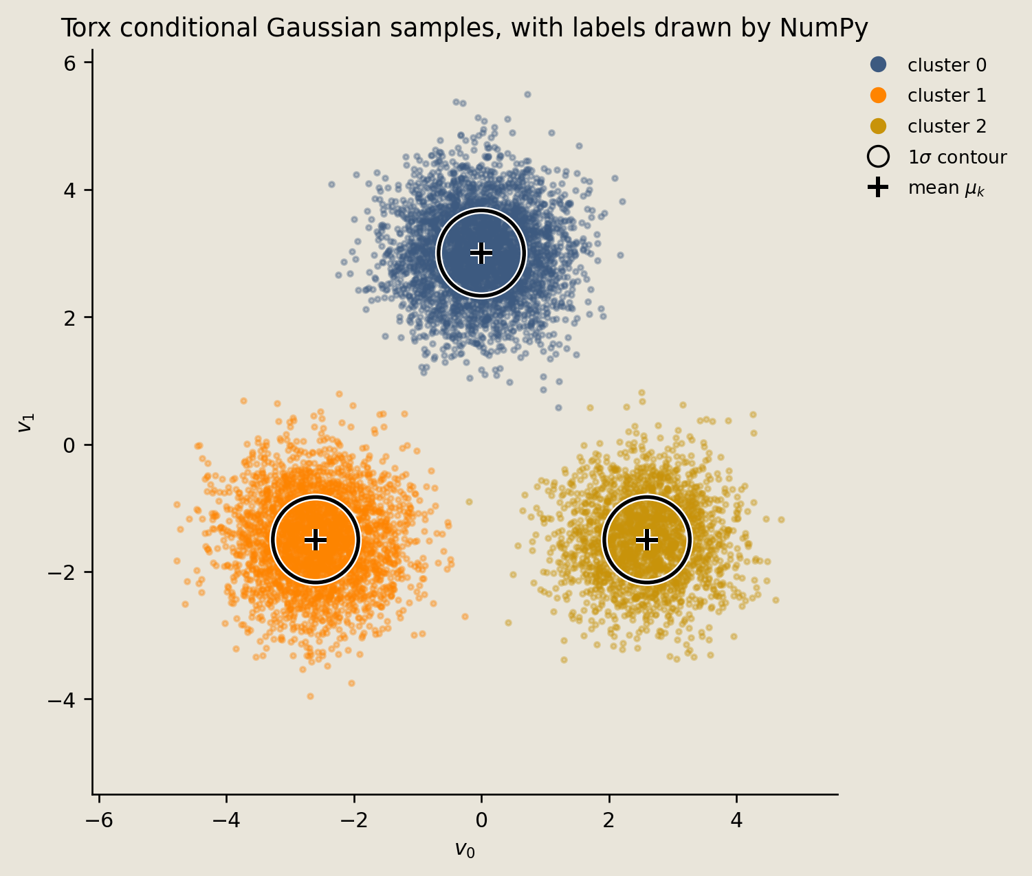
The scatter plot puts the NumPy labels and the Torx conditional samples in one frame with the analytic one-sigma contours, so we can see whether the drawn points sit where the components say they should. The black circle around each cluster is the $1\sigma$ contour of $\mathcal{N}(\mu_k,\Sigma_k)$, and the $+$ marks the mean $\mu_k$.
fig = P_fld.cluster_scatter(points, true_labels, np.asarray(cluster_means), cluster_covs)
savefig(fig, "14_generated_clusters")
Recovering clusters with the softmax
Generation fixed $h$ and sampled $v$. For recovery, we fix each observed $v$ and evaluate the other conditional:
$$ p(h=e_k\mid v)=\frac{\exp[-E_k(v)]}{\sum_{k'}\exp[-E_{k'}(v)]}=\operatorname{softmax}_k(\theta(v)),\qquad \theta_k(v)=\log \pi_k-\frac{1}{2}(v-\mu_k)^\top\Sigma_k^{-1}(v-\mu_k)-\frac{1}{2}\log\det\Sigma_k. $$
The logits are the negated component energies after removing constants shared across $k$. Their softmax is therefore both the one-hot Boltzmann conditional and the usual Gaussian-mixture responsibility.
The log-determinant is required when component covariances differ. It cancels for the shared diagonal covariance used here, but cluster_logits retains it by constructing the logits from the full component energies.
def cluster_logits(v):
    """Return the per-cluster Boltzmann logits for visible points v."""
    v = jnp.atleast_2d(jnp.asarray(v, dtype=jnp.float32))
    diff = v[:, None, :] - cluster_means[None, :, :]
    inv_vars = jnp.exp(-log_vars)
    # Lower Gaussian energy means a larger logit for that cluster. The
    # 0.5*sum(log_vars_k) component normalizer is required so marginalizing v
    # reproduces pi under per-cluster (not just shared) covariance.
    energy = (
        0.5 * jnp.sum(diff**2 * inv_vars[None, :, :], axis=-1)
        + 0.5 * jnp.sum(log_vars, axis=-1)[None, :]
        - jnp.log(pi)
    )
    return -energy
def posterior_probs(v):
    """Softmax the cluster logits into responsibilities."""
    return jax.nn.softmax(cluster_logits(v), axis=1)
posterior_probs softmaxes those logits into responsibilities, from which we take the hard label $\arg\max_k p(k\mid v)$ and the fraction of points whose top responsibility falls below 0.92, a soft-boundary score counting how many points are genuinely ambiguous. We then plot the hard labels on top of the soft responsibility field.
post_probs = np.asarray(posterior_probs(points))
hard_labels = post_probs.argmax(axis=1)
hard_accuracy = float((hard_labels == true_labels).mean())
soft_boundary_rate = float((post_probs.max(axis=1) < 0.92).mean())

print(f"hard reassignment accuracy: {hard_accuracy:.3f}")
print(f"soft boundary fraction:     {soft_boundary_rate:.3f}")
hard reassignment accuracy: 1.000
soft boundary fraction:     0.000
fig = P_fld.assignment_panels(
    points,
    true_labels,
    post_probs,
    np.asarray(cluster_means),
    posterior_fn=posterior_probs,
)
savefig(fig, "14_soft_assignment")
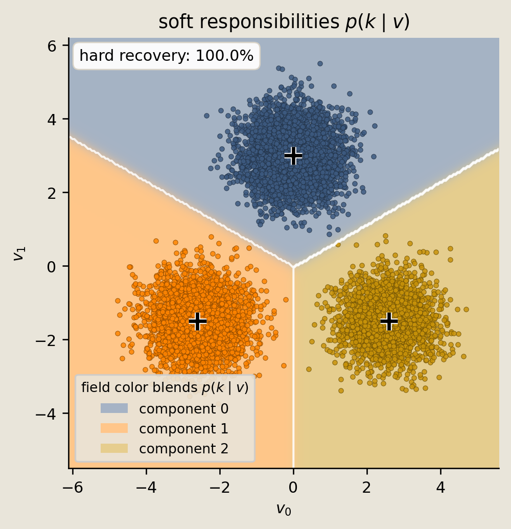
In the assignment figure, point color shows the hard label $\arg\max_k p(k\mid v)$, while the background blends component colors according to $p(k\mid v)$. The printed hard reassignment accuracy is 1.000 and the soft boundary fraction is 0.000, so every sampled point has a near-certain recovered label. The background blends only in the empty regions between clusters; it locates the decision boundary, but there are no data there on which to evaluate recovery.
One more check on the generated data closes this section. We compare the histogram of a single visible coordinate against the exact mixture density for that coordinate, which tests the marginal rather than the per-cluster blocks. The density comes from mixture_density, a notebook helper in examples/helpers/_affine_gaussian.py that evaluates the analytic Gaussian mixture on a grid.
marginal_dim = 0
grid = np.linspace(
    points[:, marginal_dim].min() - 0.7, points[:, marginal_dim].max() + 0.7, 420
)
density = np.asarray(
    mixture_density(
        cluster_means[:, marginal_dim : marginal_dim + 1],
        log_vars[:, marginal_dim : marginal_dim + 1],
        pi,
        jnp.asarray(grid),
    )
)
fig = P_fld.marginal_density(points[:, marginal_dim], grid, density)
savefig(fig, "14_marginal_density")
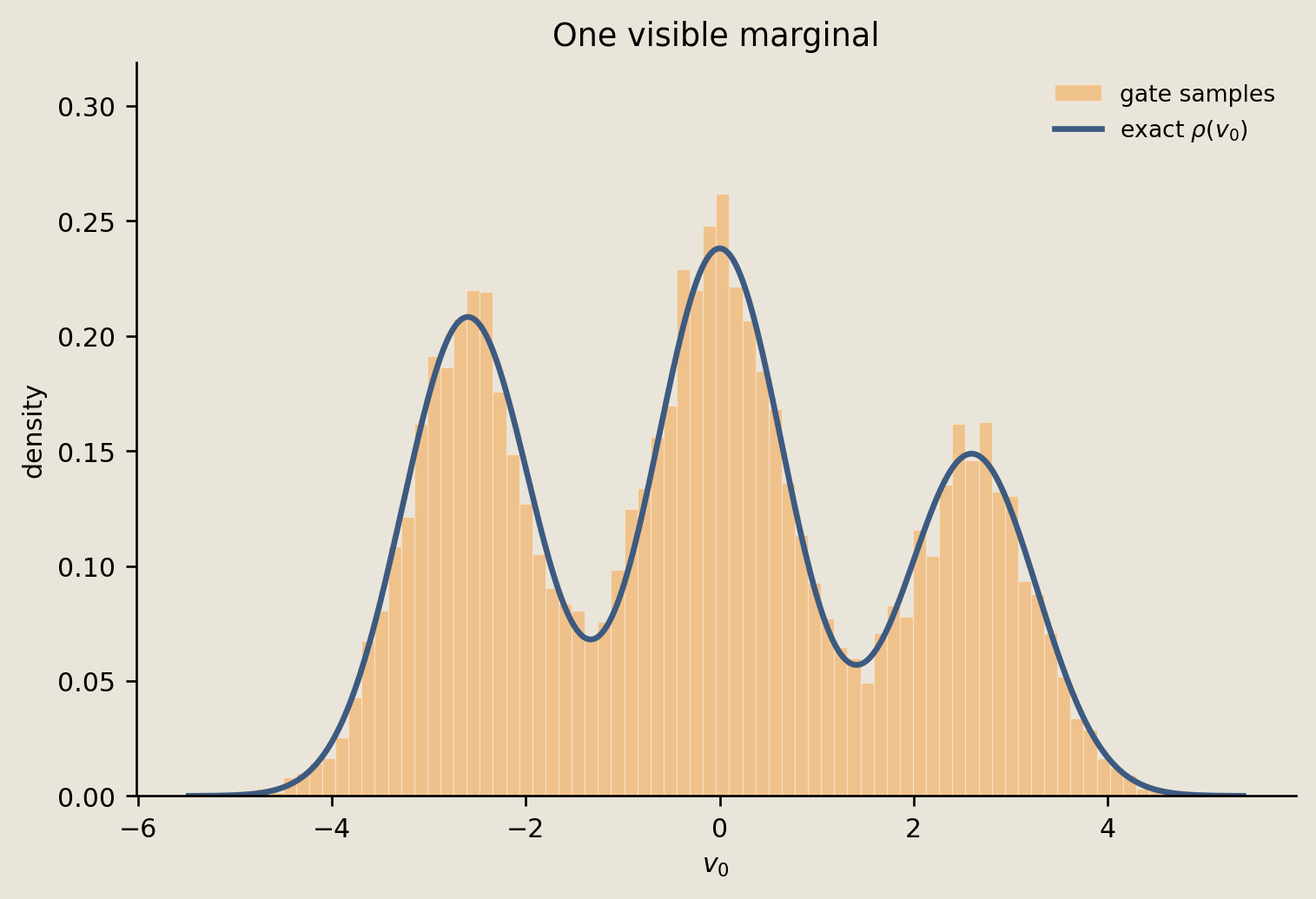
For the selected coordinate, the sampled histogram follows the analytic mixture density, so the marginal of the generated data reproduces the mixture we specified.
Block Gibbs on the joint Boltzmann machine
So far, we have used the two conditionals separately for recovery and generation. To sample the joint law, we alternate them:
$$ h\sim p(h\mid v)=\operatorname{softmax}(\theta(v)),\qquad v\sim p(v\mid h=e_k)=\mathcal{N}(v\mid\mu_k,\Sigma_k). $$
We implement both updates directly in JAX from the same formulas, leaving each step of the Gibbs procedure explicit. Torx's role in this notebook therefore ends with the conditional Gaussian draws above. During one sweep, we redraw every visible point from its current component and then redraw its label from the analytic responsibility vector.
Term: Gibbs sweep
A block Gibbs sweep (Geman and Geman 1984) redraws each variable block from its conditional distribution while holding the other block fixed.
The well-separated mixture used for clustering is a poor setting in which to study Gibbs mixing: a chain would tend to remain in its initial cluster. For the convergence study, we therefore use closer means and a larger shared variance, which makes the components overlap. Every chain starts in cluster 0, far from the target occupancy $\pi$, and we record how the population occupancy changes after each sweep. Because the population is finite, the curves will fluctuate around the dashed target values rather than match them exactly.
# the convergence study needs a mixture block Gibbs can actually mix
# on. the clustering demo above keeps well-separated means, where a chain never
# hops, so its population occupancy would be frozen by its start. these closer
# means with a larger shared variance overlap enough that the hidden block
# genuinely reassigns chains between clusters within a few tens of sweeps.
conv_means = jnp.array(
    [[0.0, 1.6], [-1.44, -0.88], [1.44, -0.88]], dtype=jnp.float32
)
conv_vars = jnp.full((K, 2), 0.9, dtype=jnp.float32)
conv_log_vars = jnp.log(conv_vars)
def conv_cluster_logits(v):
    """Per-cluster Boltzmann logits for the overlapping convergence mixture."""
    v = jnp.atleast_2d(jnp.asarray(v, dtype=jnp.float32))
    diff = v[:, None, :] - conv_means[None, :, :]
    inv_vars = jnp.exp(-conv_log_vars)
    # per-cluster log-det normalizer so the logits stay valid GMM responsibilities.
    energy = (
        0.5 * jnp.sum(diff**2 * inv_vars[None, :, :], axis=-1)
        + 0.5 * jnp.sum(conv_log_vars, axis=-1)[None, :]
        - jnp.log(pi)
    )
    return -energy
conv_sigma = jnp.sqrt(jnp.exp(conv_log_vars))


def gibbs_visible_step(labels, key):
    """Visible block: draw each chain directly from its component Gaussian."""
    mu = conv_means[labels]
    sigma = conv_sigma[labels]
    return mu + sigma * jax.random.normal(key, mu.shape)
def gibbs_hidden_step(v, key):
    """Hidden block: draw labels from the analytic GMM logits."""
    return jax.random.categorical(key, conv_cluster_logits(v), axis=1)
def _occupancy(labels, num_clusters):
    """Fraction of chains currently in each cluster."""
    return jnp.bincount(labels, length=num_clusters) / labels.shape[0]
@eqx.filter_jit
def run_gibbs_chain(key, num_chains, num_sweeps):
    # start every chain committed to cluster 0, so the population begins fully
    # off-stationary at (1, 0, 0). vmap is implicit (all chains are batched
    # array rows); lax.scan walks the sweeps under one compile.
    """Run block Gibbs from the all-cluster-0 start and record occupancy per sweep."""
    labels0 = jnp.zeros(num_chains, dtype=jnp.int32)

    def step(labels, key):
        kv, kh = jax.random.split(key)
        v = gibbs_visible_step(labels, kv)
        new_labels = gibbs_hidden_step(v, kh)
        return new_labels, _occupancy(new_labels, K)

    keys = jax.random.split(key, num_sweeps)
    _, swept = jax.lax.scan(step, labels0, keys)
    # prepend the seeded (1, 0, 0) start so the trace shows the full relaxation
    return jnp.concatenate([_occupancy(labels0, K)[None, :], swept], axis=0)
We run 30 Gibbs sweeps over 6,000 chains and record the occupancy at each sweep, which gives us the whole relaxation curve rather than only its endpoint.
N_GIBBS = 6_000
NUM_SWEEPS = 30

gibbs_occupancy = np.asarray(
    run_gibbs_chain(jax.random.key(SEED + 900), N_GIBBS, NUM_SWEEPS)
)
gibbs_sweeps = np.arange(len(gibbs_occupancy))
# the equilibrium check pools the back half, after the transient relaxes
gibbs_back_half = gibbs_occupancy[len(gibbs_occupancy) // 2 :].mean(axis=0)

print(f"start occupancy:     {gibbs_occupancy[0].round(3).tolist()}")
print(f"back-half occupancy: {gibbs_back_half.round(3).tolist()}")
print(f"target weights pi:   {np.asarray(pi).round(3).tolist()}")
start occupancy:     [1.0, 0.0, 0.0]
back-half occupancy: [0.40299999713897705, 0.3499999940395355, 0.2460000067949295]
target weights pi:   [0.4000000059604645, 0.3499999940395355, 0.25]
fig = P_samp.gibbs_convergence(gibbs_sweeps, gibbs_occupancy, np.asarray(pi))
savefig(fig, "14_gibbs_convergence")
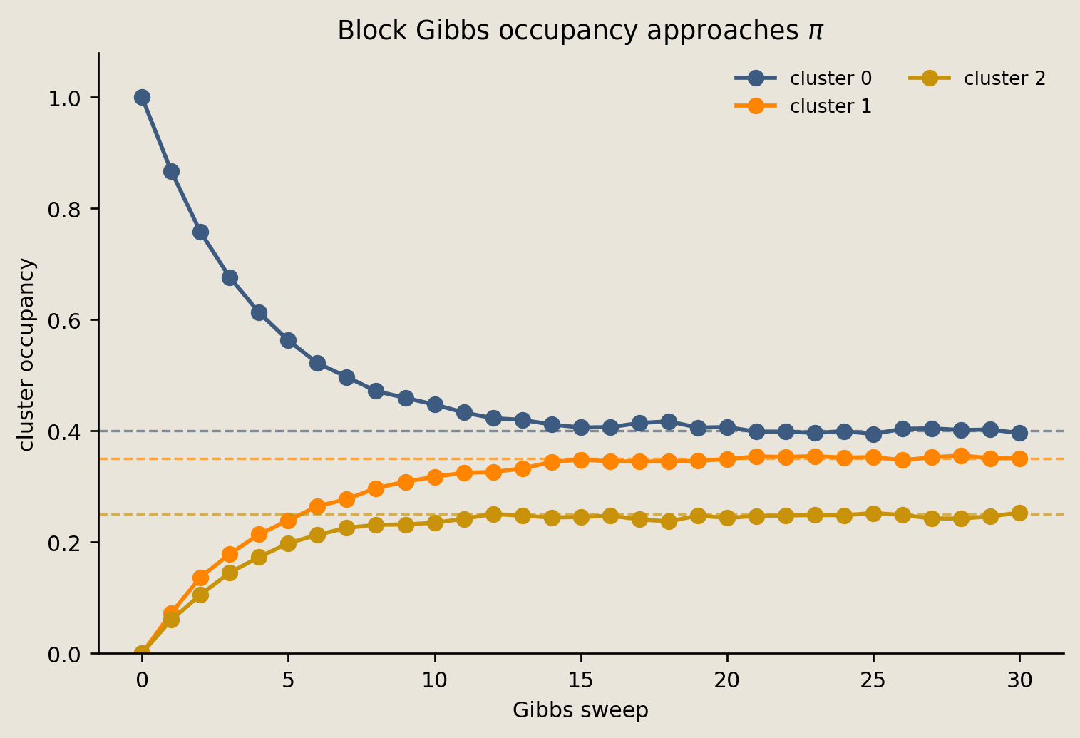
The occupancy moves away from the seeded $(1, 0, 0)$ state within a few sweeps and then fluctuates around a stable level. Averaging over the back half, after the transient, gives $(0.403, 0.350, 0.246)$ compared with $\pi=(0.400, 0.350, 0.250)$. The largest difference is 0.004, consistent with finite-population sampling noise in this experiment.
The one-hot constraint as a winner-take-all energy
The pdit used above represents only valid categorical states. What changes if we instead represent the component choice with $K$ binary units? We can favor one-hot configurations $z\in\{0,1\}^K$ with the penalty
$$ E_{\mathrm{WTA}}(z) = \lambda\Big(\sum_k z_k - 1\Big)^2, $$
whose ground states are exactly the one-hot vectors $e_k$. Up to the constant $\lambda$, this energy expands into a bias term $-\lambda\sum_k z_k$ and an all-pairs repulsion $2\lambda\sum_{k<k'} z_k z_{k'}$, giving a winner-take-all Potts-type coupling.
The Boltzmann distribution $p(z)\propto e^{-E_{\mathrm{WTA}}(z)}$ assigns equal probability to the one-hot states by symmetry. However, at finite $\lambda$ it also assigns probability to non-one-hot configurations. The energetic construction therefore matches a structural $K$-state pdit only as $\lambda\to\infty$, or after restricting the state space to the one-hot subset. Increasing $\lambda$ concentrates more probability on that subset.
We enumerate all $2^K$ binary configurations and compute their exact finite Boltzmann probabilities. This removes sampling error from the comparison. The same penalty can be realized on hardware with pairwise couplings, but the object evaluated below is the equilibrium energy distribution itself.
wta_K = 3
wta_lambda = 4.0
# Enumerate every binary configuration so the finite distribution is exact.
wta_configs = np.array(list(np.ndindex(*(2,) * wta_K)), dtype=np.int32)
wta_config_labels = np.array(["".join(map(str, z)) for z in wta_configs])
wta_is_onehot = wta_configs.sum(axis=1) == 1
With only $2^K$ configurations to sum over, the normalized Boltzmann probability of each one follows directly from its penalty energy.
def wta_probabilities(lam):
    energies = lam * (wta_configs.sum(axis=1) - 1) ** 2
    weights = np.exp(-energies)
    return weights / weights.sum(), energies
We evaluate that distribution at $\lambda=4$ and total the mass sitting on one-hot states, which is the number that says how closely the penalty imitates a pdit.
wta_probs, wta_energies = wta_probabilities(wta_lambda)
wta_onehot_mass = float(wta_probs[wta_is_onehot].sum())
wta_onehot_probs = wta_probs[wta_is_onehot]

wta_lambdas = np.linspace(0.0, 6.0, 25)
wta_onehot_sweep = np.array(
    [wta_probabilities(lam)[0][wta_is_onehot].sum() for lam in wta_lambdas]
)

print(f"lambda = {wta_lambda:.1f}")
print(f"P(one-hot) = {wta_onehot_mass:.6f}")
print("per-one-hot probabilities:", np.round(wta_onehot_probs, 6).tolist())
lambda = 4.0
P(one-hot) = 0.976161
per-one-hot probabilities: [0.325387, 0.325387, 0.325387]
fig = P_samp.winner_take_all(
    wta_config_labels,
    wta_probs,
    wta_is_onehot,
    wta_lambdas,
    wta_onehot_sweep,
)
savefig(fig, "14_winner_take_all_energy")
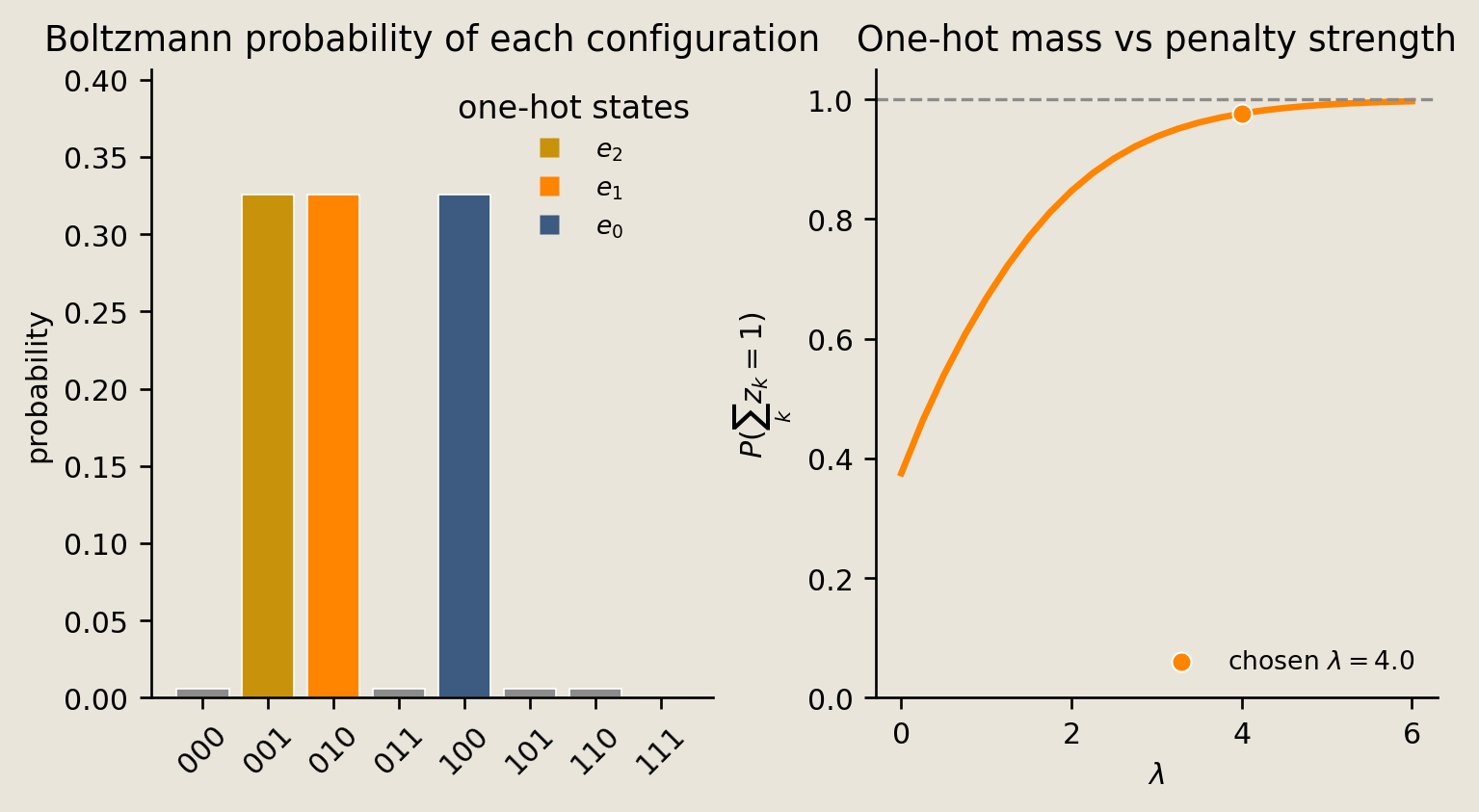
At $\lambda=4$, the three one-hot states have equal probability, 0.325387 each, and together carry 0.976161 of the total mass. The sweep shows this total increasing with $\lambda$. The remaining 0.024 lies on configurations that a $K$-state pdit cannot represent, which is the finite-strength difference between the energetic and structural encodings.
Verification
We finish by checking the numerical claims used to interpret the figures.
For generation, each cluster's sampled mean matches $\mu_k$ within 0.06, its sampled variance matches $\sigma_k^2$ within 12% relative, and the realized label proportions match $\pi$ within 0.025. These checks cover the NumPy-and-Torx conditional sampling path.
For recovery, every responsibility row sums to one within $10^{-6}$. The softmax of the Boltzmann logits also matches responsibilities computed independently from the per-component Gaussian densities within $10^{-4}$, checking that the energy and mixture calculations agree. Hard reassignment accuracy is above 0.99 for these well-separated clusters.
The pooled sample mean and variance of the visible data match the analytic mixture moments within 0.08 and 5% relative, respectively. This checks the full marginal in addition to the individual component blocks.
For the Gibbs chain, the seeded start has more than 95% of chains in cluster 0, and every component of the back-half occupancy lies within 0.04 of $\pi$. Together, these conditions distinguish relaxation from a chain initialized at its target.
Finally, the winner-take-all distribution places more than 95% of its mass on one-hot states, divides that mass equally to within $10^{-9}$, and increases it monotonically with $\lambda$. These are the three properties used in the structural-versus-energetic comparison.
for k in range(K):
    mask = true_labels == k
    np.testing.assert_allclose(
        points[mask].mean(axis=0), np.asarray(cluster_means[k]), atol=0.06
    )
    np.testing.assert_allclose(
        points[mask].var(axis=0), np.asarray(cluster_vars[k]), rtol=0.12
    )
np.testing.assert_allclose(sample_props, np.asarray(pi), atol=0.025)
np.testing.assert_allclose(post_probs.sum(axis=1), 1.0, atol=1e-6)

# energy-to-responsibility equivalence: softmax of the Boltzmann logits must
# equal the GMM responsibilities built directly from per-component densities.
ref_comp = np.stack(
    [
        np.asarray(pi[k])
        * np.exp(
            -0.5
            * np.sum(
                (points - np.asarray(cluster_means[k])) ** 2
                / np.asarray(cluster_vars[k]),
                axis=1,
            )
        )
        / np.sqrt(np.prod(2 * np.pi * np.asarray(cluster_vars[k])))
        for k in range(K)
    ],
    axis=1,
)
ref_resp = ref_comp / ref_comp.sum(axis=1, keepdims=True)
np.testing.assert_allclose(post_probs, ref_resp, atol=1e-4)

assert hard_accuracy > 0.99, f"hard assignment accuracy too low: {hard_accuracy:.3f}"
analytic_mean = np.asarray((pi[:, None] * cluster_means).sum(axis=0))
analytic_second = np.asarray(
    (pi[:, None] * (cluster_vars + cluster_means**2)).sum(axis=0)
)
analytic_var = analytic_second - analytic_mean**2
np.testing.assert_allclose(points.mean(axis=0), analytic_mean, atol=0.08)
np.testing.assert_allclose(points.var(axis=0), analytic_var, rtol=0.05)
# the chain genuinely starts off-stationary (all mass in cluster 0) and relaxes
assert gibbs_occupancy[0, 0] > 0.95, (
    f"Gibbs chain not seeded off-stationary: start {gibbs_occupancy[0].round(3)}"
)
max_gibbs_dev = float(np.max(np.abs(gibbs_back_half - np.asarray(pi))))
assert max_gibbs_dev < 0.04, f"Gibbs occupancy deviation {max_gibbs_dev:.4f} >= 0.04"
assert wta_onehot_mass > 0.95, f"WTA one-hot mass {wta_onehot_mass:.6f} <= 0.95"
np.testing.assert_allclose(wta_onehot_probs, wta_onehot_probs[0], atol=1e-9)
assert np.all(np.diff(wta_onehot_sweep) >= -1e-12), "WTA one-hot mass is not monotone"
print("all checks passed")
all checks passed
Conclusion
We began with one joint energy over a continuous visible vector and a categorical hidden state. Fixing the visible vector produced the softmax responsibilities used for clustering, while fixing the hidden state produced the component Gaussian used for generation. These are complementary conditionals of the same Gaussian-categorical Boltzmann machine.
The analytic energy and the JAX logits share the parameterization $(\mu_k,\Sigma_k,\pi_k)$, allowing the two calculations to be compared directly. NumPy drew labels and shuffled the component blocks, Torx Mixture drew the conditional Gaussian samples, and JAX recovered the responsibilities and hard assignments. Alternating the same two conditional formulas in a handwritten JAX Gibbs loop then recovered the mixture weights from an off-stationary population.
The final comparison separated two ways to encode the categorical state. A pdit enforces the $K$ valid choices structurally, whereas a finite winner-take-all energy over $K$ binary units retains some probability on invalid configurations. The latter approaches the former as the penalty strength increases.
See also:
10_pmode_gaussian_gates.ipynb, pure Gaussian gates and closed-form Gaussian conditioning.13_regime_switching_diffusion.ipynb,pdit-selected Gaussian increments in a hybrid process.
References
- Ackley, D.H., Hinton, G.E., Sejnowski, T.J. 1985. A learning algorithm for Boltzmann machines. Cognitive Science 9(1), 147-169. Foundational Boltzmann-machine definition and equilibrium treatment.
- Dempster, A.P., Laird, N.M., Rubin, D.B. 1977. Maximum likelihood from incomplete data via the EM algorithm. Journal of the Royal Statistical Society B 39(1), 1-38. Introduces the responsibility, the posterior over mixture components used throughout this notebook.
- Geman, S., Geman, D. 1984. Stochastic relaxation, Gibbs distributions, and the Bayesian restoration of images. IEEE Transactions on Pattern Analysis and Machine Intelligence 6(6), 721-741. Introduces Gibbs sampling as stochastic relaxation toward a Boltzmann distribution, the block sweep run above.