
Stochastic convolutional networks
We train a shared stochastic kernel to classify 4x4 bars-and-stripes images. param_map ties 60 physical gates to 5 trainable logits, and param_shift_inf supplies gradients estimated from samples, so the whole layer trains through the sampler. We check one shared-logit gradient against a finite-difference probe and record a six-example validation trace with seed 123.
Bars-and-stripes images differ in a simple but spatial way: rows are constant in one class, while columns are constant in the other. How can a stochastic circuit detect this distinction using the same local computation across a $4\times4$ image?
We begin with a small probabilistic kernel that acts on adjacent horizontal pixels. It plays the role of a CNN filter, except that its gates fire randomly rather than computing a fixed dot product. Each image is represented by 16 probabilistic bits (p-bits), one Bernoulli-valued state per pixel, so the layer is a parametrised stochastic circuit over those p-bits.
The convolutional structure comes from reusing one set of kernel parameters at every horizontal position. Two PCNOT pooling stages then collect the resulting state at a small set of readout sites. Because the kernel is reused across columns but not rows, this is a convolution-like stencil with horizontal weight sharing rather than a fully shift-symmetric convolution.
This tutorial uses Torx, JAX, Equinox, Optax, NumPy, and Matplotlib. It assumes basic familiarity with binary classifiers and gradients.
What runs where?
- Torx:
SampleSimulatorruns and differentiates the stochastic feature circuit. - Notebook code: Equinox supplies the linear classifier, JAX supplies transformations, and Optax applies Adam updates.
- Helpers:
examples/helpers/_notebook_paths.pyandexamples/helpers/_notebook_style.pyhandle paths and style.examples/helpers/_plots_schematics.pyandexamples/helpers/_plots_training.pydraw the figures.
We will construct the four-gate kernel (PJUMP, PReset, PNOT, PJUMP), use param_map to tie 60 physical gate positions to 5 logits, and train those logits end to end with a sample-based parameter-shift gradient and Adam. Finally, we will compare one gradient with a finite-difference estimate to check the differentiable path through the sampler.
Setup
We start with path handling, NumPy, and the notebook helpers that style and save figures consistently.
from pathlib import Path
import sys

import numpy as np
ROOT = Path.cwd()
if not (ROOT / "helpers").exists() and (ROOT.parent / "helpers").exists():
    ROOT = ROOT.parent
HELPER_DIR = ROOT / "helpers"
sys.path.insert(0, str(HELPER_DIR))
from jax.scipy.special import logit
from _notebook_paths import figure_dir
from _notebook_style import apply_notebook_style, make_savefig
import _plots_schematics as P_sch
import _plots_training as P_train

FIGURE_DIR = figure_dir(ROOT)
apply_notebook_style()


savefig = make_savefig(FIGURE_DIR)
The second import block brings in the gate primitives from torx.psc together with Equinox, JAX, and Optax, and it fixes SEED = 123. That single seed drives the data split, the classifier initialization, and every sampler key below, so every number this notebook prints is reproducible.
import itertools

import equinox as eqx
import jax
import jax.numpy as jnp
import optax
from torx.psc import (
    DiscretePCircuit,
    PCNOT,
    PJUMP,
    PNOT,
    PReset,
    BranchingSimulator,
)

SEED = 123
rng = np.random.default_rng(SEED)
The dataset
Bars-and-stripes is a small binary image set whose two classes differ only in whether rows or columns are constant, which makes it a fair test for a layer built out of horizontal neighbour interactions.
An image is a bar when every row is uniform, so it reads as horizontal bands, and a stripe when every column is uniform, so it reads as vertical stripes. The all-zero and all-one images satisfy both definitions, and the helper below keeps those duplicates as bars by convention, which yields 16 bars and 14 stripes. With seed 123 we split the 30 distinct patterns into 24 training examples and 6 validation examples, and the same six validation examples are scored after every epoch.
bars_and_stripes builds the labeled set by enumerating every constant-row pattern as a bar and every constant-column pattern as a stripe, skipping images it has already seen so the two uniform patterns are counted once. We then fix N_SIDE = 4 and materialize the flattened patterns and labels arrays.
def bars_and_stripes(n):
    patterns, labels = [], []
    # Keep uniform duplicates as bars.
    seen = set()
    for rows in itertools.product([0, 1], repeat=n):
        # Bars: constant rows (repeat one column vector across all columns).
        image = np.repeat(np.array(rows)[:, None], n, axis=1)
        key = tuple(image.reshape(-1))
        if key not in seen:
            patterns.append(image.reshape(-1))
            labels.append(0)
            seen.add(key)
    for cols in itertools.product([0, 1], repeat=n):
        # Stripes: constant columns (repeat one row vector across all rows).
        image = np.repeat(np.array(cols)[None, :], n, axis=0)
        key = tuple(image.reshape(-1))
        if key not in seen:
            patterns.append(image.reshape(-1))
            labels.append(1)
            seen.add(key)
    return np.asarray(patterns, dtype=np.int32), np.asarray(labels, dtype=np.float32)
N_SIDE = 4
N_PBITS = N_SIDE * N_SIDE
patterns, labels = bars_and_stripes(N_SIDE)
The class counts are the first thing a bug in that enumeration would break, so we assert them before anything else uses the data: 30 distinct patterns, 16 pixels each, 16 bars and 14 stripes. Double-counted uniform images fail here rather than surface later as a mislabeled batch.
n_bars = int((labels == 0).sum())
n_stripes = int((labels == 1).sum())

assert len(patterns) == 30, f"expected 30 patterns, got {len(patterns)}"
assert patterns.shape[1] == N_PBITS
assert (n_bars, n_stripes) == (16, 14)
assert n_bars + n_stripes == 30

print(f"dataset: {len(patterns)} patterns  ({n_bars} bars, {n_stripes} stripes)")
dataset: 30 patterns (16 bars, 14 stripes)
Building the kernel circuit
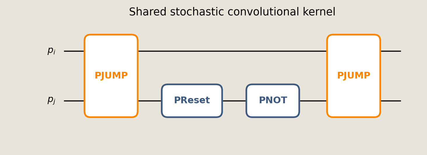
The circuit has two kinds of repeated structure. First, a local kernel applies four gates—PJUMP, PReset, PNOT, and PJUMP—to each adjacent horizontal pixel pair. The 12 applications occupy different sites, but param_map assigns their corresponding gates to the same kernel logits. Thus every pair is processed by the same learned stochastic operation, as pixels at different locations share a filter in a CNN. Since the reuse is horizontal only, the resulting stencil is convolution-like but does not have exact shift symmetry, and there is no shared vertical kernel.
Second, column-then-row PCNOT pooling reduces the 16 p-bits to 4 readout sites and introduces two additional shared logits.
To count the parameters, consider what one logit controls. Each gate is a convex combination of the identity and a deterministic operation $B$, applied with probability $\sigma(\theta)$:
$$G(\theta)=\underbrace{(1-\sigma(\theta))\,I}_{\vphantom{\big|}\text{do nothing}}+\underbrace{\sigma(\theta)\,B}_{\vphantom{\big|}\text{apply }B}.$$
Here $\sigma(\theta)=1/(1+e^{-\theta})$ is the gate-on probability. The two PJUMP gates in the local kernel share logit 0, so its 4 gates require only 3 logits. The two pooling stages contribute 2 more, giving 5 trainable logits for 60 physical gates.
build_scnn_circuit lays out the shared kernel and the two pooling stages in one pass, appending a param_map entry next to every gate it creates, so the tying is written down in the same place as the wiring instead of being reconstructed afterwards.
def build_scnn_circuit():
    """Construct the shared-kernel SCNN circuit, parameter map, and readout sites."""
    gates = []
    param_map = []
    # Shared local stochastic convolution on adjacent horizontal pairs.
    for r in range(N_SIDE):
        for c in range(N_SIDE - 1):
            i = r * N_SIDE + c
            j = i + 1
            gates.extend(
                [
                    PJUMP([i, j]),
                    PReset(j),
                    PNOT(j),
                    PJUMP([j, i]),
                ]
            )
            # These four physical gates read from three shared kernel logits.
            param_map.extend([0, 1, 2, 0])
    # Pool adjacent columns, then adjacent rows of the pooled sites.
    pooled = []
    for r in range(N_SIDE):
        for c in range(0, N_SIDE, 2):
            src = r * N_SIDE + c
            sink = src + 1
            gates.append(PCNOT([src, sink]))
            param_map.append(3)
            pooled.append(sink)
    readout_sites = []
    for c in range(2):
        for r in range(0, N_SIDE, 2):
            src = pooled[r * 2 + c]
            sink = pooled[(r + 1) * 2 + c]
            gates.append(PCNOT([src, sink]))
            param_map.append(4)
            readout_sites.append(sink)
    return DiscretePCircuit(gates), np.asarray(param_map), readout_sites
Building the circuit hands us the gate list, the param_map, and the 4 readout sites. We then choose the five starting values as gate-on probabilities, because probabilities are easier to reason about than logits, and pass them through jax.scipy.special.logit, the inverse sigmoid, to get the logits the model actually trains.
circuit, param_map, readout_sites = build_scnn_circuit()
initial_gate_logits = jnp.asarray(
    [logit(0.34), logit(0.08), logit(0.06), logit(0.55), logit(0.60)]
)
The logit accounting above is easy to get wrong, so we assert it against the circuit we just built: 60 physical gates, 4 readout sites, and 5 distinct entries in param_map. A miscounted loop shows up here as a failed assertion instead of a silent shape mismatch further down.
assert len(circuit.gates) == 60, f"expected 60 gates, got {len(circuit.gates)}"
assert len(readout_sites) == 4
assert len(np.unique(param_map)) == 5

print(f"circuit: {len(circuit.gates)} gates, {len(np.unique(param_map))} shared logits")
print(f"readout sites: {readout_sites}")
circuit: 60 gates, 5 shared logits
readout sites: [5, 13, 7, 15]
We first draw the local kernel by itself, where the four-gate sequence is easiest to inspect. Orange denotes the two-site PJUMP coupling gates; slate denotes the single-site PReset and PNOT gates. This view shows the operation applied at one location, but not yet how its parameters are reused across the grid.
kernel = DiscretePCircuit(circuit.gates[:4])
fig = P_sch.plot_kernel_circuit(kernel)
savefig(fig, "08_scnn_circuit")
To show that reuse, we next draw the full circuit and encode the positions governed by each of its five logits. The schematic recovers the spatial wiring from circuit and param_map rather than declaring it separately, so it displays the sharing present in the constructed circuit.
The 16 p-bits occupy a $4\times4$ grid. Each horizontal pair receives the same local kernel, after which two stages of PCNOT pooling collect the state at 4 readout sites. Gold and copper distinguish the two pooling stages.
# Recover the spatial wiring from the circuit + param_map for the schematic.
def _gate_sites(g):
    return [int(v) for v in g.sites]
conv_pairs, _seen = [], set()
col_pool_edges, row_pool_edges = [], []
for g, p in zip(circuit.gates, param_map):
    if p not in (0, 3, 4):
        continue
    s = _gate_sites(g)
    if p == 0 and len(s) == 2:  # PJUMP conv gate -> horizontal pixel pair
        pair = tuple(sorted(s))
        if pair not in _seen:
            _seen.add(pair)
            conv_pairs.append(pair)
    elif p == 3:  # stage-1 column pooling PCNOT
        col_pool_edges.append((s[0], s[1]))
    elif p == 4:  # stage-2 row pooling PCNOT
        row_pool_edges.append((s[0], s[1]))
fig = P_sch.plot_weight_sharing_schematic(
    N_SIDE,
    conv_pairs,
    col_pool_edges,
    row_pool_edges,
    readout_sites,
    len(circuit.gates),
    len(np.unique(param_map)),
)
savefig(fig, "08_weight_sharing")
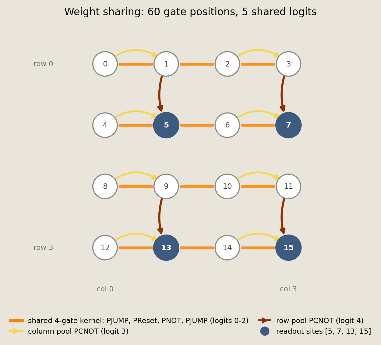
Every gate position drawn with the same line style and color is driven by the same logit, so only five parameter groups are free in the entire layer, and the dark nodes mark the four readout sites the classifier will see.
Training the kernel
Training requires derivatives of expectations produced by a sampler. A parameter-shift estimator obtains these derivatives without differentiating the discrete sampling operation: it evaluates the circuit with a gate parameter fixed at special values and combines the resulting expectations.
We use Branching with diff_method="param_shift_inf" and num_samples=256. For a gate $G(\theta)=(1-\sigma(\theta))I+\sigma(\theta)B$, the special values are the two logit limits, $-\infty$ and $+\infty$, which deterministically select the identity branch and the $B$ branch.
For a readout $O$, the derivative of the expected readout with respect to the gate logit is
$$ \frac{\mathrm{d}}{\mathrm{d}\theta}\,\mathbb E[O]\;=\;\sigma(\theta)\,\bigl(\mathbb E[O\mid B]-\mathbb E[O]\bigr), $$
where the two clamps provide the branch expectations $\mathbb E[O\mid I]$ and $\mathbb E[O\mid B]$, and $\mathbb E[O]=(1-\sigma(\theta))\,\mathbb E[O\mid I]+\sigma(\theta)\,\mathbb E[O\mid B]$ is the expectation under the current circuit. Each expectation is estimated from samples, so the gradient contains Monte Carlo noise. We will measure its agreement with a finite difference below. Unlike the finite-shift quantum rules in Mitarai et al. (2018) and Schuld et al. (2019), this classical stochastic rule evaluates the two deterministic branches directly.
Rebuilding the circuit on every forward pass would repeat work that never changes, so we build the differentiable sampler sim once and compile the circuit once into scnn_template. Each forward pass then uses eqx.tree_at to swap the current shared logits into that template, which keeps the gate thetas tied to the trainable logits.
sim = BranchingSimulator(diff_method="param_shift_inf", num_samples=256)
# compile the structure-only circuit once; the forward pass swaps in the
# current shared logits with eqx.tree_at instead of rebuilding the circuit.
# num_samples comes from the calling sampler, so this template is reusable by
# the finite-difference sampler too.
scnn_template = sim.build_circuit(circuit, [jnp.zeros((1,)) for _ in circuit.gates])
SCNN implements the sharing as an array operation. Indexing the 5 shared logits by param_map expands them to the 60 gate positions. During differentiation, contributions from every position assigned to the same index accumulate into that shared logit. The sampler returns expected p-bit values, and only the 4 readout sites are passed to the linear sigmoid classifier.
class SCNN(eqx.Module):
    gate_logits: jax.Array
    linear: eqx.nn.Linear
    # non-inexact: adam skips structural indices
    _param_map: jax.Array
    _readout_sites_arr: jax.Array

    def __call__(self, x, key, sampler):
        # Broadcast the 5 shared logits onto the 60 physical gate positions.
        full_thetas = self.gate_logits[self._param_map][:, None]
        # Swap the shared logits into the precompiled template instead of
        # rebuilding the circuit; keeps the thetas tied to the trainable logits.
        compiled = eqx.tree_at(lambda c: c.thetas, scnn_template, full_thetas)
        ev = sampler.expval_all(compiled, x, key)
        # The classifier sees only the pooled readout sites.
        features = ev[self._readout_sites_arr]
        return jax.nn.sigmoid(jnp.squeeze(self.linear(features)))
We draw the train-validation split once from rng with seed 123. The same 6 images are therefore evaluated after every epoch, rather than changing with the training randomness. We also compute the validation majority baseline: the accuracy obtained by always predicting the more frequent class among those 6 images.
order = rng.permutation(len(patterns))
train_idx, val_idx = order[:24], order[24:]
x_train = jnp.asarray(patterns[train_idx])
y_train = jnp.asarray(labels[train_idx])
x_val = jnp.asarray(patterns[val_idx])
y_val = jnp.asarray(labels[val_idx])
train_n, val_n = len(x_train), len(x_val)
assert train_n == 24 and val_n == 6
val_class_counts = np.bincount(np.asarray(y_val, dtype=np.int32), minlength=2)
val_majority_count = int(val_class_counts.max())
val_majority_acc = val_majority_count / val_n
print(f"train / validation split (seed {SEED}): {train_n} / {val_n}")
print(
    f"validation majority baseline: {val_majority_count} of {val_n} "
    f"({val_majority_acc:.0%})"
)
train / validation split (seed 123): 24 / 6
validation majority baseline: 4 of 6 (67%)
model = SCNN(
    gate_logits=initial_gate_logits,
    linear=eqx.nn.Linear(len(readout_sites), 1, key=jax.random.key(SEED)),
    _param_map=jnp.asarray(param_map),
    _readout_sites_arr=jnp.asarray(readout_sites),
)
Adam at a learning rate of 5e-2 does the updating, and eqx.filter(model, eqx.is_inexact_array) decides what it may touch: the 5 shared logits and the linear head, but not the integer param_map and readout indices, which are structure rather than parameters.
optimizer = optax.adam(5e-2)
opt_state = optimizer.init(eqx.filter(model, eqx.is_inexact_array))
The objective is binary cross-entropy over the batch. Predictions are clipped away from 0 and 1 so that the logarithms remain finite. Applying eqx.filter_value_and_grad to bce_loss propagates the parameter-shift derivative through the sampler and returns gradients with respect to the shared logits. We retain the undecorated bce_loss because the finite-difference calculation later needs loss values without gradients.
The remaining wrappers separate the two operations used in each epoch: train_step computes one Adam update, while evaluate returns validation loss and accuracy without changing the parameters.
def bce_loss(model, x_batch, y_batch, key, sampler=sim):
    # Give each image its own random key for independent sampler noise.
    keys = jax.random.split(key, len(x_batch))
    preds = jax.vmap(lambda xi, ki: model(xi, ki, sampler))(x_batch, keys)
    preds = jnp.clip(preds, 1e-6, 1.0 - 1e-6)
    return jnp.mean(
        -(y_batch * jnp.log(preds) + (1.0 - y_batch) * jnp.log(1.0 - preds))
    )


# undecorated bce_loss is reused by the finite-difference probe (loss only);
# this wrapper adds the param-shift gradient for training and the analytic check
loss_fn = eqx.filter_value_and_grad(bce_loss)
@eqx.filter_jit
def train_step(model, opt_state, x_batch, y_batch, key):
    loss, grads = loss_fn(model, x_batch, y_batch, key)
    updates, opt_state = optimizer.update(
        grads, opt_state, eqx.filter(model, eqx.is_inexact_array)
    )
    model = eqx.apply_updates(model, updates)
    return model, opt_state, loss
@eqx.filter_jit
def evaluate(model, x_batch, y_batch, key, sampler=sim):
    keys = jax.random.split(key, len(x_batch))
    preds = jax.vmap(lambda xi, ki: model(xi, ki, sampler))(x_batch, keys)
    preds = jnp.clip(preds, 1e-6, 1.0 - 1e-6)
    loss = jnp.mean(
        -(y_batch * jnp.log(preds) + (1.0 - y_batch) * jnp.log(1.0 - preds))
    )
    acc = jnp.mean((preds >= 0.5) == y_batch)
    return loss, acc
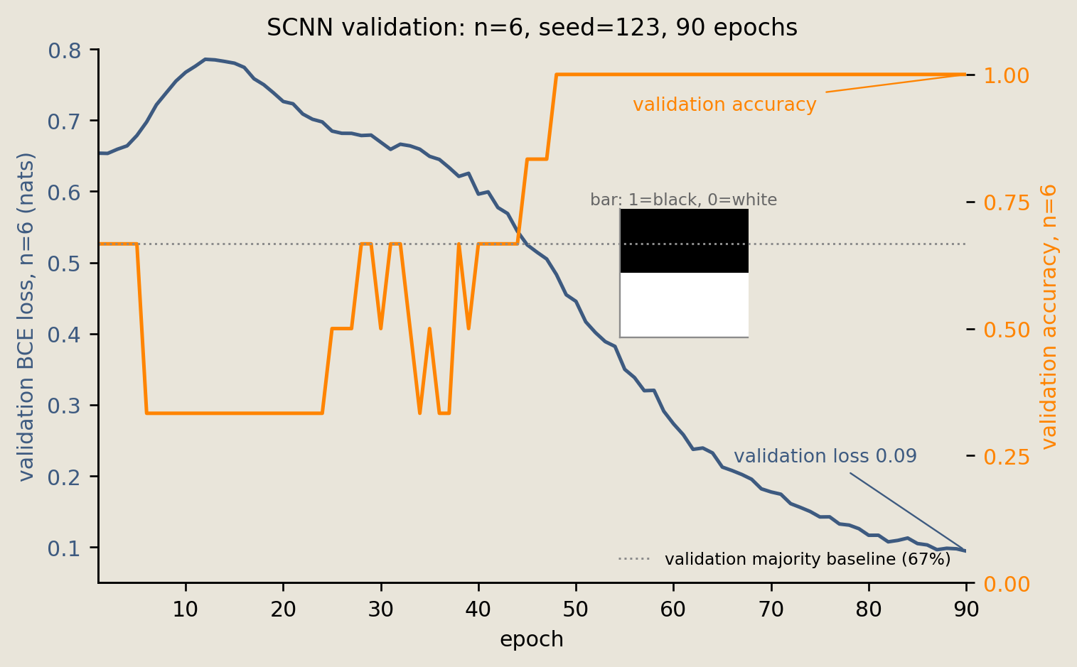
We train for 90 full-batch epochs. At each epoch, fit_model splits the seed-123 key into independent keys for the training update and validation evaluation, so their sampler estimates do not reuse the same random draws. The function records validation loss and accuracy on the fixed six-example set, after which we report the final values for n=6.
def fit_model(model, opt_state, x_train, y_train, x_val, y_val):
    loss_history, acc_history = [], []
    key = jax.random.key(SEED)
    for epoch in range(90):
        # Split once per epoch so training and validation use independent samples.
        key, train_key, eval_key = jax.random.split(key, 3)
        model, opt_state, _ = train_step(model, opt_state, x_train, y_train, train_key)
        val_loss, val_acc = evaluate(model, x_val, y_val, eval_key)
        # keep device arrays; convert the whole trace to host once after training
        loss_history.append(val_loss)
        acc_history.append(val_acc)
    return model, opt_state, np.asarray(loss_history), np.asarray(acc_history)
model, opt_state, loss_history, acc_history = fit_model(
    model, opt_state, x_train, y_train, x_val, y_val
)

print(f"final validation loss (n={val_n}):     {loss_history[-1]:.4f}")
print(f"final validation accuracy (n={val_n}): {acc_history[-1]:.2%}")
final validation loss (n=6):     0.0944
final validation accuracy (n=6): 100.00%
For this fixed seed, the six-item validation set ends at 100% accuracy, which is a coarser claim than it sounds, because with six examples accuracy can only change in increments of $1/6$.
Gradient check
The existence of a gradient does not establish that its value is correct. We therefore examine one shared PJUMP logit (LOGIT_IDX = 0) by comparing its param_shift_inf gradient with a central finite-difference estimate. Both calculations use the same small batch of 4 bars and 4 stripes. Because both expectations are sample estimates, agreement is required only within 30% relative error. The check covers one of the five logits, so it tests the wiring of one differentiable path rather than verifying every parameter.
LOGIT_IDX = 0
bars_idx = np.where(labels == 0)[0][:4]
stripes_idx = np.where(labels == 1)[0][:4]
batch_x = jnp.asarray(patterns[np.concatenate([bars_idx, stripes_idx])])
batch_y = jnp.asarray(labels[np.concatenate([bars_idx, stripes_idx])])
key_grad = jax.random.key(SEED + 7)

_, grads = loss_fn(model, batch_x, batch_y, key_grad)
g_analytic = float(grads.gate_logits[LOGIT_IDX])
The reference calculation is a central finite difference of the loss with respect to the same logit. It does not invoke the parameter-shift gradient code, so agreement compares two independent derivative constructions. fd_grad creates a Branching with the requested sample count for each probe, allowing later probes to reduce sampling noise.
def fd_grad(m, epsilon, n_samples):
    fd_sampler = BranchingSimulator(diff_method="param_shift_inf", num_samples=n_samples)
    m_plus = eqx.tree_at(
        lambda mod: mod.gate_logits,
        m,
        m.gate_logits.at[LOGIT_IDX].add(epsilon),
    )
    m_minus = eqx.tree_at(
        lambda mod: mod.gate_logits,
        m,
        m.gate_logits.at[LOGIT_IDX].add(-epsilon),
    )
    # Reuse key_grad on both sides so only the logit perturbation changes.
    # bce_loss (undecorated) computes loss only, so no param-shift gradient is
    # wasted on each finite-difference evaluation.
    loss_plus = float(bce_loss(m_plus, batch_x, batch_y, key_grad, fd_sampler))
    loss_minus = float(bce_loss(m_minus, batch_x, batch_y, key_grad, fd_sampler))
    return (loss_plus - loss_minus) / (2.0 * epsilon)
We now compare the estimates. A finite difference computed from samples can miss the tolerance because of Monte Carlo noise, so we try probes with 256, 1024, and 2048 samples per side, stopping at the first relative error below REL_ERR_TOL = 0.30. The following assertion applies the same threshold. This procedure distinguishes a persistent disagreement from the scatter of a single finite-sample probe, while retaining the stated 30% tolerance.
print(f"analytic (param-shift, logit {LOGIT_IDX}): {g_analytic:.6f}")
REL_ERR_TOL = 0.30
FD_PROBES = [(256, 0.05), (1024, 0.05), (2048, 0.10)]
g_fd, rel_err = None, np.inf
for i, (n_samples, eps) in enumerate(FD_PROBES):
    g_fd = fd_grad(model, eps, n_samples)
    rel_err = abs(g_analytic - g_fd) / (abs(g_fd) + 1e-6)
    label = "finite-diff" if i == 0 else "retry finite-diff"
    print(f"{label} (eps={eps}, {n_samples} samples/side): {g_fd:.6f}")
    print(f"relative error: {rel_err:.4f}")
    if rel_err < REL_ERR_TOL:
        break
analytic (param-shift, logit 0): -0.013853
finite-diff (eps=0.05, 256 samples/side): -0.016632
relative error: 0.1671
assert (
    rel_err < REL_ERR_TOL
), f"gradient check failed: analytic={g_analytic}, fd={g_fd}, rel_err={rel_err}"
print(f"gradient check passed (rel_err < {REL_ERR_TOL:.2f})")
gradient check passed (rel_err < 0.30)
Kernel parameter shifts
Validation accuracy alone cannot show that the stochastic kernel was trained, because the linear head might improve while the kernel remains at its initial values. We therefore compare the initial and trained logits for each shared gate. The checks require an L2 shift above 1e-3, a maximum absolute shift above 0.05, and final accuracy of at least 0.75. Nonzero movement in the gate logits establishes that the gradient reached the shared kernel, although it does not by itself identify which learned settings caused the accuracy change.
gate_names = ["PJUMP", "PReset", "PNOT", "PCNOT-col", "PCNOT-row"]

print(f"{'gate':<12}  {'init logit':>10}  {'trained logit':>13}  {'shift':>8}")
print("-" * 48)
for name, init_l, fin_l in zip(
    gate_names, initial_gate_logits.tolist(), model.gate_logits.tolist()
):
    print(f"{name:<12}  {init_l:>10.4f}  {fin_l:>13.4f}  {fin_l - init_l:>+8.4f}")

gate_shift = float(jnp.linalg.norm(model.gate_logits - initial_gate_logits))
max_abs_shift = float(jnp.max(jnp.abs(model.gate_logits - initial_gate_logits)))

print(f"\nL2 shift: {gate_shift:.4f}    max |shift|: {max_abs_shift:.4f}")

assert acc_history[-1] >= 0.75, f"accuracy {acc_history[-1]:.2%} below 0.75 threshold"
assert gate_shift > 1e-3, "gate logits did not move during training"
assert (
    max_abs_shift > 0.05
), f"max logit shift {max_abs_shift:.4f} < 0.05, gradient did not reach the kernel"
print("\nall checks passed")
print("  acc_history[-1] >= 0.75")
print("  gate logit L2 shift > 1e-3")
print("  max |gate logit shift| > 0.05")
gate          init logit  trained logit     shift
------------------------------------------------
PJUMP            -0.6633         0.1162   +0.7795
PReset           -2.4423        -5.6673   -3.2249
PNOT             -2.7515        -6.2989   -3.5474
PCNOT-col         0.2007         3.6767   +3.4760
PCNOT-row         0.4055        -2.8612   -3.2667
L2 shift: 6.8078    max |shift|: 3.5474

all checks passed
  acc_history[-1] >= 0.75
  gate logit L2 shift > 1e-3
  max |gate logit shift| > 0.05
Training curve
The final figure shows the quantities evaluated after every epoch: validation BCE and validation accuracy on the same six examples. Since accuracy changes by $1/6$ for each corrected example, its panel forms a staircase. The 67% line marks the majority-class accuracy for this seed-specific validation split, and the inset encodes black pixels as 1 and white pixels as 0. Because the six images are evaluated repeatedly rather than reserved as an untouched test set, these curves describe optimization on a fixed validation set; they are not an independent estimate of generalization.
# Pick a visually informative bar pattern: top two rows black, bottom two white.
bar_idx = next(
    i
    for i, (p, l) in enumerate(zip(patterns, labels))
    if l == 0 and tuple(p.reshape(N_SIDE, N_SIDE)[:, 0]) == (1, 1, 0, 0)
)
bar_image = patterns[bar_idx].reshape(N_SIDE, N_SIDE)
fig = P_train.plot_training_curve(
    loss_history,
    acc_history,
    bar_image,
    validation_n=val_n,
    majority_baseline=val_majority_acc,
    title=f"SCNN validation: n={val_n}, seed={SEED}, 90 epochs",
)
savefig(fig, "08_scnn_training")
print(f"final validation accuracy: {acc_history[-1]:.2%}")
print(f"gate logit L2 shift:       {gate_shift:.4f}")
print(f"max |gate logit| shift:    {max_abs_shift:.4f}")
final validation accuracy: 100.00%
gate logit L2 shift:       6.8078
max |gate logit| shift:    3.5474
Conclusion
We have constructed a stochastic convolutional network over 16 p-bits, one per pixel, and trained it to classify bars-and-stripes images by differentiating expected readouts from the sampler.
- A four-gate kernel (
PJUMP,PReset,PNOT,PJUMP) is applied to every adjacent horizontal pixel pair, followed byPCNOTpooling to 4 readout sites. param_mapties the 60 physical gates to 5 shared logits. This parameter reuse defines a convolution-like horizontal stencil, but not exact shift symmetry.param_shift_infestimates gradients through the sampler, andoptax.adamupdates the shared logits and linear head together.- A central finite-difference probe compares one shared
PJUMPgradient with theparam_shift_infestimate on one small batch, using a 30% tolerance. This supports the differentiable path for that logit without constituting a full five-logit verification.
The next notebook, 09_stochastic_graph_networks.ipynb, applies another shared-parameter learning pattern to a stochastic graph circuit.
References
- Mitarai, K., Negoro, M., Kitagawa, M., Fujii, K. 2018. Quantum circuit learning. Phys. Rev. A 98, 032309.
- Schuld, M., Bergholm, V., Gogolin, C., Izaac, J., Killoran, N. 2019. Evaluating analytic gradients on quantum hardware. Phys. Rev. A 99, 032331.