
Posterior per-pixel denoising on MNIST
An offline UNet supplies clean-pixel probabilities, and Torx draws each output pixel through one PNOT gate. We show one genuine Torx draw separately from a thresholded 64-draw ensemble estimator. The committed FID numbers (Fréchet inception distance, a standard score for generated images) describe the offline UNet checkpoint and not anything Torx produced here.
Discrete diffusion begins with a process we can specify exactly: starting from a clean binary image, independently flip its pixels until the image is corrupted. The reverse problem is less direct. Given the corrupted image $x_t$, how can we turn a denoiser's beliefs about the clean pixels into a stochastic step that Torx can execute?
We use the independent bit-flip process of Austin et al. 2021, written as the continuous-time Markov chain of Campbell et al. 2022, to define the corruption. This forward process provides the context rather than the method executed by the circuit. The computation we run is narrower: a host UNet estimates $\hat p_i = P(x_{0,i}=1 \mid x_t)$ for each pixel, and Torx independently resamples the pixels from those posterior probabilities.
Each binary pixel is therefore a probabilistic bit, or pbit, which is the unit sampled by Torx. A single PNOT gate maps the current pixel and its corresponding probability to a Bernoulli draw with parameter $\hat p_i$.
The UNet has 472,545 parameters and was trained offline. We load its committed weights and evaluation artifacts rather than training it on this page, which keeps the example fast but also limits what it can establish: the repository does not contain the training and FID evaluation script, so this notebook cannot reproduce the checkpoint's training split or FID protocol.
We will:
- set up the forward bit-flip kernel and load the committed corrupted MNIST batch,
- map the UNet's per-pixel clean probabilities to one
PNOTlogit per pbit, - compare one stochastic Torx draw with a thresholded 64-draw ensemble estimator, and
- keep the eight-image display-batch error separate from the offline UNet artifact metrics.
Setup
We import the local helpers, set the plotting style, and fix the random seed so every draw below repeats exactly.
from pathlib import Path
import sys
import json

import equinox as eqx
import jax
import jax.numpy as jnp
import numpy as np
ROOT = Path.cwd()
if not (ROOT / "helpers").exists() and (ROOT.parent / "helpers").exists():
    ROOT = ROOT.parent
HELPER_DIR = ROOT / "helpers"
sys.path.insert(0, str(HELPER_DIR))
from _notebook_style import (
    apply_notebook_style,
    make_savefig,
)
from _notebook_paths import asset_dir, figure_dir
from _plots_schematics import draw_pcircuit
from _nb07_diffusion import (
    denoise_logits,
    frechet_distance,
    load_unet_params,
    pca_features,
)
from _plots_training import (
    plot_diffusion_loss,
    plot_fid_drop,
    plot_flip_probability,
    plot_reconstruction_grid,
)

from torx.psc import DiscretePCircuit, PNOT, BranchingSimulator
apply_notebook_style()
FIGURE_DIR = figure_dir(ROOT)
ASSET_DIR = asset_dir(ROOT, "nb07")
savefig = make_savefig(FIGURE_DIR)

SEED = 123
Loading the checkpoint and evaluation grids
Everything the denoiser knows was learned before this page ran, so the first job is to load it. The committed artifacts under assets/nb07/ hold the UNet parameters, the saved training loss, the evaluation grids, and sparse run metadata.
What runs where?
- Torx: 784
PNOTgates and stochastic sampling. - Notebook code: probability-to-logit mapping, display-batch metrics, and PCA-space comparison.
examples/helpers/_nb07_diffusion.py: host UNet inference and PCA/Fréchet calculations.examples/helpers/_plots_training.py: figures only.- Offline assets: metadata, evaluation grids, loss history, and UNet weights, all committed to the repository without the script that produced them.
The helper load_unet_params in examples/helpers/_nb07_diffusion.py rebuilds the UNet from those committed weights.
meta = json.loads((ASSET_DIR / "meta.json").read_text())
grids = np.load(ASSET_DIR / "eval_grids.npz")
loss_history = np.load(ASSET_DIR / "loss_history.npy")
# init the frozen UNet structure, then fill it from the committed msgpack
params = load_unet_params(ASSET_DIR / "unet_mnist.msgpack")
clean_all = grids["clean"].astype(np.int32)
noisy_all = grids["noisy"].astype(np.int32)
denoised_all = grids["denoised"].astype(np.int32)
# the checkpoint was scored at this single corruption level: a per-bit flip
# probability (the forward process flips each pixel independently with this prob)
forward_p = float(meta["p_flip"])
print(
    f"UNet: {meta['n_params']:,} params, {meta['n_steps']:,} steps, "
    f"final loss {meta['final_loss']:.3f}"
)
print(f"dataset: {meta['dataset']}")
print(f"eval grids: clean / noisy / denoised, each {clean_all.shape}")
UNet: 472,545 params, 30,000 steps, final loss 0.183
dataset: mnist_784 binarized@0.5, 28x28, 70k
eval grids: clean / noisy / denoised, each (64, 28, 28)
Binarized pixels as pbits
To interpret the reverse step, we first specify the corruption it is meant to undo. We represent a binary image with one pbit for each pixel.
The forward process is a continuous-time Markov chain: a random process that jumps between states at random times. For a single pixel, the uniform rate matrix below defines the shared flip rate:
$$ Q = \begin{pmatrix} -1 & 1 \\ 1 & -1 \end{pmatrix}. $$
At noise time $\sigma$, exponentiating this rate matrix gives the transition kernel:
$$ e^{\sigma Q} = \begin{pmatrix} \tfrac12 + \tfrac12 e^{-2\sigma} & \tfrac12 - \tfrac12 e^{-2\sigma} \\[3pt] \tfrac12 - \tfrac12 e^{-2\sigma} & \tfrac12 + \tfrac12 e^{-2\sigma} \end{pmatrix}. $$
The off-diagonal entry $\tfrac12(1 - e^{-2\sigma})$ is the probability that a bit has flipped by time $\sigma$; the diagonal entry $\tfrac12(1 + e^{-2\sigma})$ is the probability that it remains unchanged. At $\sigma = 0$, no bits have flipped. As $\sigma \to \infty$, the flip probability approaches $\tfrac12$, and the initial bit is lost in pure noise.
The committed noisy grids use the checkpoint's evaluation level, forward_p = 0.30: each pixel in a clean MNIST image is flipped independently with probability 0.30. We next select eight images for display, then compare this specified rate with the bit error observed in that batch.
n_show = 8
clean = clean_all[:n_show]
noisy = noisy_all[:n_show]
denoised = denoised_all[:n_show]

height, width = clean.shape[1:]
num_bits = height * width
Before building any circuit we confirm that the eight-image display batch really is binary and $28\times28$, and that the observed corruption matches the stated rate. Every bit-error value in this notebook is measured on these eight images alone.
assert np.all((clean == 0) | (clean == 1))
assert np.all((noisy == 0) | (noisy == 1))
assert (height, width) == (28, 28)

print(f"image size: {height}x{width} = {num_bits} bits per image")
print(f"forward bit-flip rate: {forward_p}")
print(f"observed forward bit error: {float(np.mean(noisy != clean)):.3f}")
image size: 28x28 = 784 bits per image
forward bit-flip rate: 0.3
observed forward bit error: 0.301
The following plot shows how the flip probability changes with noise time and marks the corruption level used by the checkpoint.
fig = plot_flip_probability(forward_p)
savefig(fig, "07_flip_probability")
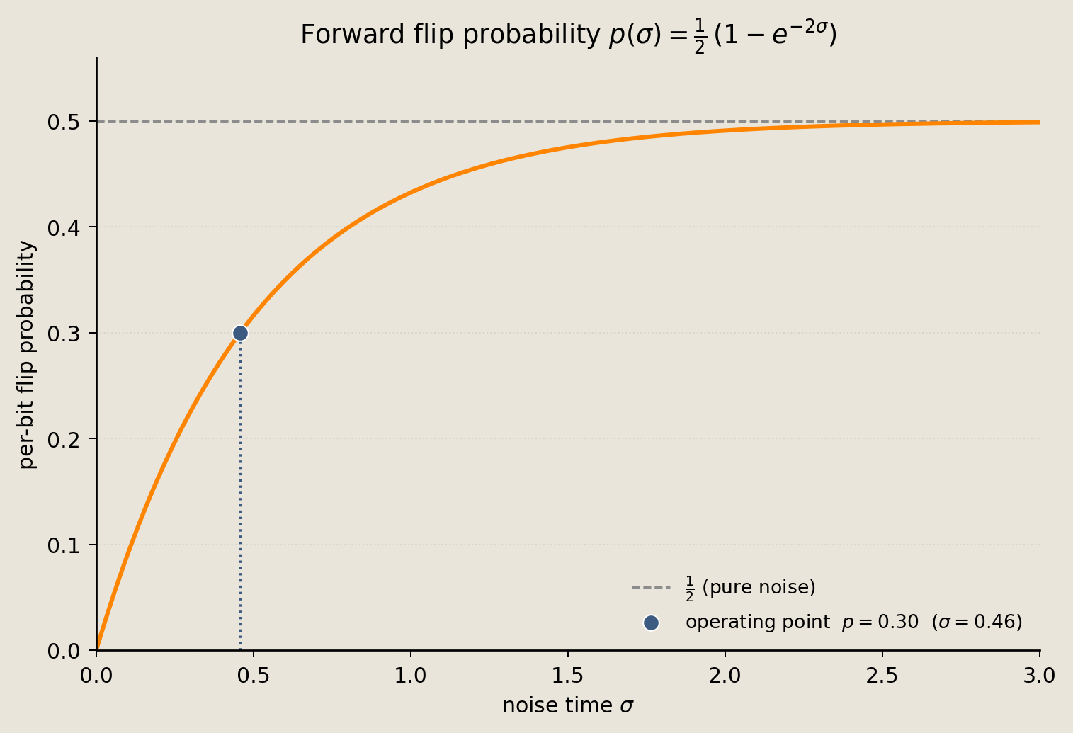
At the marked level of 0.30 the curve is still well below the 0.5 pure-noise limit, so the corrupted images retain enough signal for the reverse step to work with.
Posterior clean-bit probabilities
The forward kernel tells us how pixels are corrupted, but it does not by itself tell a gate which clean value to sample. That information comes from the host denoiser.
The denoiser is a 472,545-parameter UNet with two downsampling blocks, a bottleneck, and two upsampling blocks with skip connections. Each block uses two GroupNorm-normalized $3\times3$ convolutions, and the final per-pixel sigmoid output $\hat p_i$ estimates $P(x_{0,i}=1 \mid x_t)$. Its definition and loader are in examples/helpers/_nb07_diffusion.py. This establishes the division of computation used throughout the notebook: the offline UNet computes the posterior probabilities, while Torx samples the output bits.
PNOT is parameterized by a flip probability rather than a clean-pixel probability. For current pixel $x_{t,i}$, we therefore set
$$ p^{(i)}_{\text{flip}} = \begin{cases} 1 - \hat p_i & x_{t,i} = 1 \\ \hat p_i & x_{t,i} = 0. \end{cases} \qquad \theta^{(i)} = \log \frac{p^{(i)}_{\text{flip}}}{1 - p^{(i)}_{\text{flip}}}. $$
This mapping has the same interpretation for either input value. When the input is 0, the output becomes 1 exactly when PNOT flips; when the input is 1, the output remains 1 exactly when it does not flip. In both cases, the output bit is Bernoulli($\hat p_i$).
The resulting construction performs posterior per-pixel denoising rather than sampling from a joint time-transition kernel derived from the forward process. Its limitation is explicit: neighboring pixels do not move jointly within a reverse step. In exchange, the circuit uses only one gate per pbit.
Saved training loss
The checkpoint's metadata records 30,000 offline gradient steps, and the loss history from that run is committed alongside the weights. We plot it to see how the offline training ended, with the dashed line marking the final saved value of 0.183.
fig = plot_diffusion_loss(loss_history, reference_loss=meta["final_loss"])
savefig(fig, "07_diffusion_training_loss")
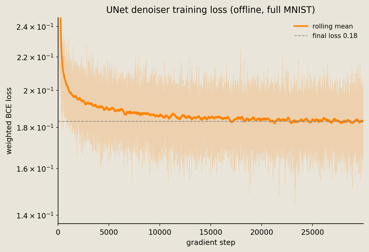
The curve flattens near the saved value by step 30,000, showing that the recorded training loss changed little near the end of the run. It does not establish convergence or generalization: the committed artifacts include neither a validation loss nor a stopping rule, and they omit the training script needed to examine either claim.
The posterior per-pixel circuit
Now we build the circuit that turns those probabilities into pixels. One PNOT gate per pixel draws independently from the UNet's clean-bit marginal, which is why the reverse step here has no time-step size and no neighbor-conditioned joint transition to configure.
The cell below wraps the helper's host UNet forward pass, denoise_logits, into a per-pixel clean-probability function.
def predict_clean_probability(batch, sigma):
    """Per-pixel clean probabilities from the offline-trained UNet."""
    # the denoiser reads both the noisy pixels and the current noise level
    logits = denoise_logits(params, batch.astype(np.float32), sigma)
    return np.asarray(jax.nn.sigmoid(logits))
We draw four wires instead of 784 so the repeating gate pattern stays legible.
demo_specs = [
    ("PNOT", [0]),
    ("PNOT", [1]),
    ("PNOT", [2]),
    ("PNOT", [3]),
]
fig = draw_pcircuit(
    demo_specs,
    wire_labels=[r"$p_0$", r"$p_1$", r"$p_2$", r"$p_3$"],
    title="Posterior denoising: one PNOT per pixel",
)
savefig(fig, "07_posterior_circuit")
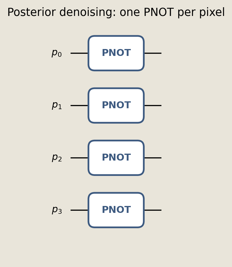
Each wire carries one independent posterior draw, and the full circuit tiles this same pattern across all 784 pixels.
We next assemble the 784-gate circuit template. eqx.filter_jit compiles the vmap-batched sampler once, after which every image reuses it and the build cost is paid only once. The num_draws argument controls how to interpret the returned mean. With one draw, the mean is the binary sample itself; with multiple independent draws, it is a Monte Carlo estimate of each pixel's posterior marginal.
def torx_posterior_mean(batch, *, seed_offset=0, num_draws=1):
    """Return the mean of independent Torx posterior per-pixel draws."""
    x = batch.reshape(len(batch), -1).astype(np.int32)
    n_pixels = x.shape[1]
    sim = BranchingSimulator(num_samples=num_draws)

    gates = [PNOT(i) for i in range(n_pixels)]
    init_thetas = [jnp.zeros((1,)) for _ in gates]
    template = sim.build_circuit(DiscretePCircuit(gates), init_thetas)

    def sample_one(row, row_p, row_key):
        pnot_thetas = jnp.log(row_p / (1.0 - row_p))[:, None]
        compiled = eqx.tree_at(lambda c: c.thetas, template, pnot_thetas)
        return sim.sample(compiled, row, row_key).mean(axis=0)

    sample_batch = eqx.filter_jit(jax.vmap(sample_one))

    # Convert the committed per-bit corruption probability to CTMC time for
    # the host UNet conditioning channel: p = 0.5 * (1 - exp(-2 sigma)).
    sigma = -0.5 * float(np.log1p(-2 * forward_p))
    clean_prob = jnp.asarray(
        predict_clean_probability(x.reshape(len(batch), height, width), sigma)
    ).reshape(len(batch), -1)
    xj = jnp.asarray(x)
    p_flip = jnp.where(xj == 1, 1.0 - clean_prob, clean_prob)
    keys = jax.random.split(jax.random.key(SEED + seed_offset), len(x))
    mean = sample_batch(xj, p_flip, keys)
    return np.asarray(mean).reshape(batch.shape)
# With one draw, the returned mean is the genuine binary Torx sample itself.
torx_draw = torx_posterior_mean(noisy, seed_offset=10, num_draws=1).astype(np.int32)

# This separate run estimates each posterior marginal with 64 Torx draws.
torx_ensemble_mean = torx_posterior_mean(noisy, seed_offset=11, num_draws=64)
# Thresholding the 64-draw mean yields an ensemble posterior-mode estimator,
# not one stochastic sample.
torx_ensemble_binary = (torx_ensemble_mean >= 0.5).astype(np.int32)
forward_display_error = float(np.mean(noisy != clean))
unet_display_error = float(np.mean(denoised != clean))
torx_draw_display_error = float(np.mean(torx_draw != clean))
torx_ensemble_display_error = float(np.mean(torx_ensemble_binary != clean))

assert torx_ensemble_display_error < forward_display_error, (
    f"ensemble estimator must reduce display-batch error: "
    f"forward={forward_display_error:.3f}, ensemble={torx_ensemble_display_error:.3f}"
)

print("bit error on the 8-image display batch")
print(f"  forward corrupted:      {forward_display_error:.3f}")
print(f"  offline UNet threshold: {unet_display_error:.3f}")
print(f"  one Torx draw:          {torx_draw_display_error:.3f}")
print(f"  Torx 64-draw ensemble:  {torx_ensemble_display_error:.3f}")
bit error on the 8-image display batch
  forward corrupted:      0.301
  offline UNet threshold: 0.058
  one Torx draw:          0.127
  Torx 64-draw ensemble:  0.082
Draw and ensemble grid
The point of the grid below is to keep one honest sample visually separate from an estimator assembled out of many samples. Each row shows the same eight $28\times28$ binary digits at a different stage: clean, forward corrupted, the offline UNet threshold, one genuine stochastic Torx draw, and the mean of 64 separate Torx draws thresholded at 0.5. That last row is an ensemble posterior-mode estimator rather than a sample, so by construction it should look tidier than the single draw. Every printed bit-error value is scoped to these eight displayed images.
rows = [
    ("clean", clean),
    ("forward\ncorrupted", noisy),
    ("offline UNet\nthreshold", denoised),
    ("one Torx\ndraw", torx_draw),
    ("Torx 64-draw\nensemble", torx_ensemble_binary),
]
fig = plot_reconstruction_grid(rows)
savefig(fig, "07_discrete_diffusion_samples")
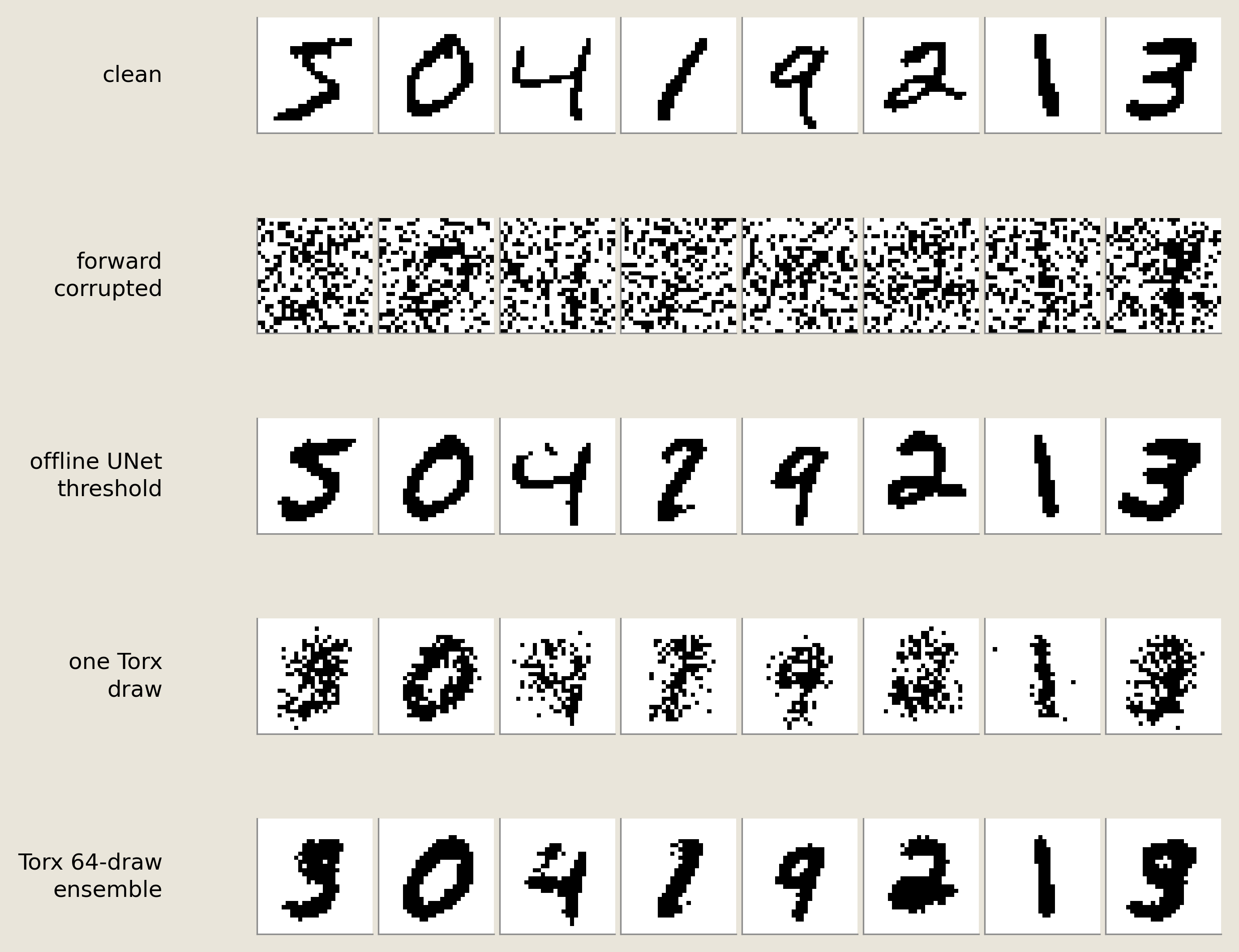
Both Torx outputs cut the bit error on this eight-image display batch, from 0.301 after corruption to 0.127 for the single draw and 0.082 for the 64-draw ensemble. The gap between those two is the sampling variation visible in the fourth row, and averaging it away is what carries the ensemble toward the 0.058 of the offline UNet threshold.
Offline UNet artifact metric
The checkpoint metadata includes FID scores from an offline evaluation. Before interpreting their change, we must specify which outputs they measure.
Fréchet inception distance fits Gaussians to Inception features from two image sets and compares those distributions; lower values indicate greater similarity in that feature space.
The committed values are 19.21 for corrupted images and 2.63 for images denoised by the offline UNet. Neither value scores a Torx draw, because the Torx outputs in this notebook were never evaluated with FID. Moreover, the artifacts omit the evaluation split, sample count, preprocessing, and FID implementation. The following figure should therefore be read as checkpoint metadata, not as a reproduced result.
fig = plot_fid_drop(
    fid_corrupted=meta["fid_corrupted"],
    fid_denoised=meta["fid_denoised"],
    title="Offline UNet checkpoint FID metadata",
)
savefig(fig, "07_discrete_diffusion_fid")
print(
    f"offline UNet metadata FID: corrupted {meta['fid_corrupted']:.2f} "
    f"-> UNet-denoised {meta['fid_denoised']:.2f}"
)
print("Torx outputs were not evaluated with FID.")
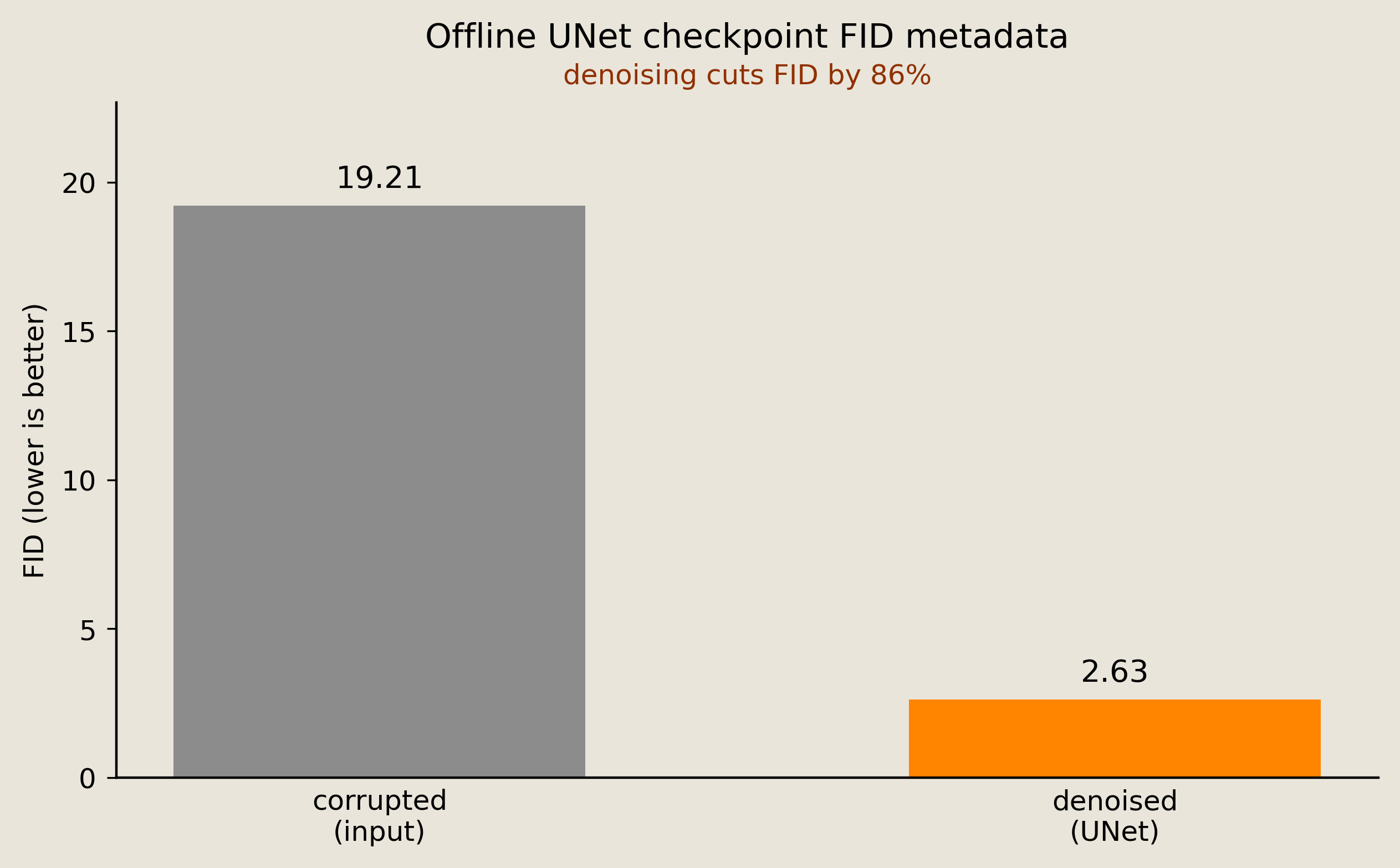
offline UNet metadata FID: corrupted 19.21 -> UNet-denoised 2.63
Torx outputs were not evaluated with FID.
Inception features come from ImageNet-like RGB images, which makes FID a poor fit for binary MNIST. As a descriptive stand-in we build a feature space the data actually occupies: we fit 16 principal components to 32 clean reference images, then compare clean, corrupted, and denoised versions of the other 32 in that space. The Fréchet distance we compute there measures how far a set's mean and covariance in those 16 coordinates sit from the clean reference set's, so it scores a distribution rather than any single image. Because the reference images are never evaluated, the two sets stay disjoint and leakage can't flatter the result.
half = len(clean_all) // 2
pca_map = pca_features(clean_all[:half], n_components=16, seed=SEED)

pca_reference = pca_map(clean_all[:half])
pca_clean_eval = pca_map(clean_all[half:])
pca_corrupted_eval = pca_map(noisy_all[half:])
pca_denoised_eval = pca_map(denoised_all[half:])

fd_clean = frechet_distance(pca_reference, pca_clean_eval)
fd_corrupted = frechet_distance(pca_reference, pca_corrupted_eval)
fd_denoised = frechet_distance(pca_reference, pca_denoised_eval)

assert fd_denoised < fd_corrupted

print("Fréchet distance in PCA-16 space (32 reference, 32 evaluation)")
print(f"  clean evaluation     : {fd_clean:6.2f}")
print(f"  corrupted evaluation : {fd_corrupted:6.2f}")
print(f"  denoised evaluation  : {fd_denoised:6.2f}")
Fréchet distance in PCA-16 space (32 reference, 32 evaluation)
  clean evaluation     :  13.86
  corrupted evaluation :  29.64
  denoised evaluation  :  14.20
Corruption pushes the evaluation set out to 29.64 in this space, while the offline UNet-denoised grids come back to 14.20, close to the 13.86 that the untouched clean images score. With 32 reference and 32 evaluation images each value is noisy, so the ordering is the part to read.
Conclusion
We ran posterior per-pixel denoising on binarized MNIST with Torx stochastic circuits, using an offline UNet for the probabilities and Torx for the randomness.
- Each $28\times28$ image uses 784
PNOTgates, one per pixel. - The host UNet supplies clean-pixel posterior probabilities, and the notebook maps them to
PNOTflip logits. - One genuine Torx draw is shown separately from the thresholded 64-draw ensemble estimator, because only the first is a sample.
- Bit error on the eight-image display batch falls from 0.301 after corruption to 0.127 for the single draw and 0.082 for the ensemble.
- The committed FID values of 19.21 and 2.63 belong to the offline UNet artifacts, and the PCA-space Fréchet check is descriptive, not FID, so no number here scores a Torx output on a generative metric.
A natural next step is 08_stochastic_convolutional_networks.ipynb, which trains stochastic image circuits with parameter-shift gradients.
References
- Austin, J., Johnson, D.D., Ho, J., Tarlow, D., van den Berg, R. 2021. Structured denoising diffusion models in discrete state-spaces. NeurIPS 34.
- Campbell, A., Benton, J., De Bortoli, V., Rainforth, T., Deligiannidis, G., Doucet, A. 2022. A continuous time framework for discrete denoising models. NeurIPS 35.